ARX Time-Series Model
ARX models are a powerful tool for modeling and analyzing the behavior of dynamic systems. They are widely used in a variety of fields, including control engineering, signal processing, and electrical engineering. ARX models are often used in control engineering, where they are used to design controllers for systems such as robots or manufacturing processes. ARX models are based on the concept of linear time-invariant (LTI) systems, which are systems that can be described by linear differential equations. In an ARX model, the input and output of a system are related by a linear equation.


An ARX model is a combination of an autoregressive model (AR) and an exogenous input model (X). It is used to represent the dynamics of a system and is commonly used in control engineering to model and analyze dynamic systems.
Autoregressive Model
An autoregressive model is a type of statistical model that represents a time series as a linear combination of its past values and a stochastic process. It is represented by the following equation:
$$y(t) = c + a_1 y(t-1) + a_2 y(t-2) + ... + a_p y(t-p) + e(t)$$
where y(t) is the value of the time series at time t, c is a constant term, a1, a2, ..., ap are the autoregressive coefficients, y(t-1), y(t-2), ..., y(t-p) are the past values of the time series, and e(t) is a random error term.
Exogenous Input
An exogenous input model represents a time series as a linear combination of its past values and a set of exogenous (i.e., external) input variables. It is represented by the following equation:
$$y(t) = c + b_1 u(t-1) + b_2 u(t-2) + ... + b_q u(t-q) + e(t)$$
where y(t) is the value of the time series at time t, c is a constant term, u(t-1), u(t-2), ..., u(t-q) are the exogenous input variables, and b1, b2, ..., bq are the coefficients that capture the relationship between the input variables and the output. The value of u(t-2) has a zero-order hold from t-2 to t-1 where the new value u(t-1) is measured or actuated.
ARX Model
An autoregressive exogenous input (ARX) model is a combination of an AR model and an X model, and it is represented by the following equation:
$$y(t) = c + a_1 y(t-1) + a_2 y(t-2) +\ldots+ a_p y(t-p) \\+ b_1 u(t-1) + b_2 u(t-2) +\ldots+ b_q u(t-q) + e(t)$$
ARX time series models are a linear representation of a dynamic system in discrete time. Putting a model into ARX form is the basis for many methods in process dynamics and control analysis. Below is the time series model with a single input and single output with k as an index that refers to the time step.
$$y_{k+1} = \sum_{i=1}^{n_a} a_i y_{k-i+1} + \sum_{i=1}^{n_b} b_i u_{k-i+1}$$
With na=3, nb=2, nu=1, and ny=1 the time series model is:
$$y_{k+1} = a_1 \, y_k + a_2 \, y_{k-1} + a_3 \, y_{k-2} + b_1 \, u_k + b_2 \, u_{k-1}$$
The time-delay between in the input and output allows the model to take into account the fact that the input and output of a system may not be perfectly synchronized in time. There may also be multiple inputs and multiple outputs such as when na=1, nb=1, nu=2, and ny=2.
$$y1_{k+1} = a_{1,1} \, y1_k + b_{1,1} \, u1_k + b_{1,2} \, u2_k$$
$$y2_{k+1} = a_{1,2} \, y2_k + b_{2,1} \, u1_k + b_{2,2} \, u2_k$$
Time series models are used for identification and advanced control. It has been in use in the process industries such as chemical plants and oil refineries since the 1980s. Model predictive controllers rely on dynamic models of the process, most often linear empirical models obtained by system identification.
Below is an overview of how to simulate and identify with ARX models using Python Gekko. There is also a Graphical User Interface (GUI) to identify models with the BYU PRISM Seeq SysID Open-Source Package.
Simulate ARX Model
 Inputs: Input (u)
 Outputs: Output (y)
 Description: ARX Time Series Model
 GEKKO Usage: y,u = m.arx(p,y=[],u=[])
from gekko import GEKKO
import matplotlib.pyplot as plt
na = 2 # Number of A coefficients
nb = 1 # Number of B coefficients
ny = 2 # Number of outputs
nu = 2 # Number of inputs
# A (na x ny)
A = np.array([[0.36788,0.36788],\
[0.223,-0.136]])
# B (ny x (nb x nu))
B1 = np.array([0.63212,0.18964]).T
B2 = np.array([0.31606,1.26420]).T
B = np.array([[B1],[B2]])
C = np.array([0,0])
# create parameter dictionary
# parameter dictionary p['a'], p['b'], p['c']
# a (coefficients for a polynomial, na x ny)
# b (coefficients for b polynomial, ny x (nb x nu))
# c (coefficients for output bias, ny)
p = {'a':A,'b':B,'c':C}
# Create GEKKO model
m = GEKKO(remote=False)
# Build GEKKO ARX model
y,u = m.arx(p)
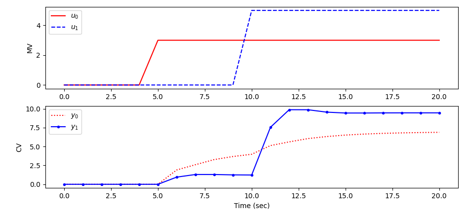
# load inputs
tf = 20 # final time
u1 = np.zeros(tf+1)
u2 = u1.copy()
u1[5:] = 3.0
u2[10:] = 5.0
u[0].value = u1
u[1].value = u2
m.time = np.linspace(0,tf,tf+1)
m.options.imode = 4
m.options.nodes = 2
m.solve()
plt.figure(1)
plt.subplot(2,1,1)
plt.plot(m.time,u[0].value,'r-',label=r'$u_0$')
plt.plot(m.time,u[1].value,'b--',label=r'$u_1$')
plt.ylabel('MV')
plt.legend(loc='best')
plt.subplot(2,1,2)
plt.plot(m.time,y[0].value,'r:',label=r'$y_0$')
plt.plot(m.time,y[1].value,'b.-',label=r'$y_1$')
plt.ylabel('CV')
plt.xlabel('Time (sec)')
plt.legend(loc='best')
plt.tight_layout()
plt.show()
Identify ARX Model
 Inputs:
   t = time data
   u = input data for the regression
   y = output data for the regression
   na = number of output coefficients (default=1)
   nb = number of input coefficients (default=1)
   nk = input delay steps (default=0)
   shift (optional) with 'none' (no shift)
                         'init' (initial pt)
                         'mean' (mean center)
                         'calc' (calculate c)
   scale (optional)
   pred (option) 'model' or 'meas'
   objf = Objective scaling factor
   diaglevel = diagnostic level (0-6)
 Outputs:
   y = predicted values
   p = ARX coefficients for m.arx()
   K = gain matrix
 Description: System Identification
 GEKKO Usage: y,p,K = sysid(t,u,y,na,nb,shift=0,pred='model',objf=1)
import pandas as pd
import matplotlib.pyplot as plt
# load data and parse into columns
url = 'http://apmonitor.com/dde/uploads/Main/tclab_step_test.txt'
data = pd.read_csv(url)
t = data['Time']
u = data[['Q1','Q2']]
y = data[['T1','T2']]
# generate time-series model
m = GEKKO(remote=False)
# system identification
na = 2 # output coefficients
nb = 2 # input coefficients
yp,p,K = m.sysid(t,u,y,na,nb)
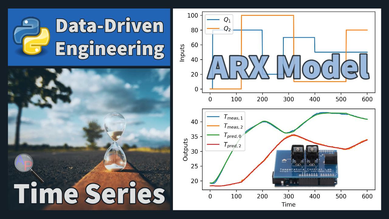
plt.figure(figsize=(8,5))
plt.subplot(2,1,1)
plt.plot(t,u)
plt.legend([r'$Q_1$',r'$Q_2$'])
plt.ylabel('Inputs')
plt.subplot(2,1,2)
plt.plot(t,y)
plt.plot(t,yp)
plt.legend([r'$T_{m,1}$',r'$T_{m,2}$',r'$T_{p,0}$',r'$T_{p,2}$'])
plt.ylabel('Outputs')
plt.xlabel('Time')
plt.tight_layout()
plt.savefig('sysid.png',dpi=300)
plt.show()
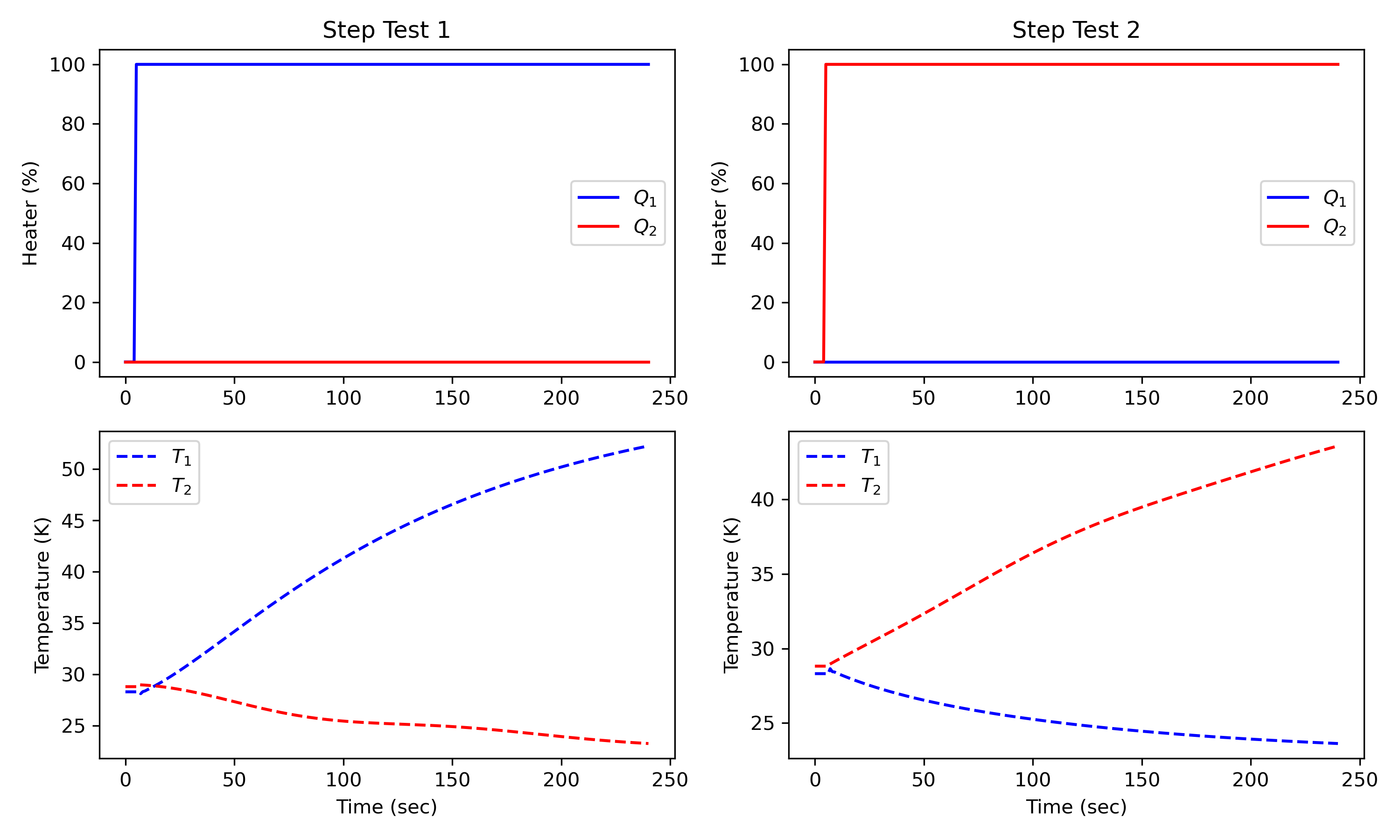
Step Test ARX Model
import numpy as np
import pandas as pd
import matplotlib.pyplot as plt
# load data and parse into columns
url = 'http://apmonitor.com/dde/uploads/Main/tclab_step_test.txt'
data = pd.read_csv(url)
t = data['Time']
u = data[['Q1','Q2']]
y = data[['T1','T2']]
# generate time-series model
m = GEKKO(remote=False)
# system identification
na = 3 # output coefficients
nb = 4 # input coefficients
yp,p,K = m.sysid(t,u,y,na,nb)
plt.figure(figsize=(8,5))
plt.subplot(2,1,1)
plt.plot(t,u)
plt.legend([r'$Q_1$',r'$Q_2$'])
plt.ylabel('Inputs')
plt.subplot(2,1,2)
plt.plot(t,y)
plt.plot(t,yp)
plt.legend([r'$T_{1,meas}$',r'$T_{2,meas}$',\
r'$T_{1,pred}$',r'$T_{2,pred}$'])
plt.ylabel('Outputs')
plt.xlabel('Time')
plt.savefig('sysid2.png',dpi=300)
# step test model
yc,uc = m.arx(p)
# steady state initialization
m.options.IMODE = 1
m.solve(disp=False)
# dynamic simulation (step tests)
m.time = np.linspace(0,240,241)
m.options.TIME_SHIFT=0
m.options.IMODE = 4
m.solve(disp=False)
plt.figure(figsize=(10,6))
# step for first MV (Heater 1)
uc[0].value = np.zeros(len(m.time))
uc[0].value[5:] = 100
uc[1].value = np.zeros(len(m.time))
m.solve(disp=False)
plt.subplot(2,2,1)
plt.title('Step Test 1')
plt.plot(m.time,uc[0].value,'b-',label=r'$Q_1$')
plt.plot(m.time,uc[1].value,'r-',label=r'$Q_2$')
plt.ylabel('Heater (%)')
plt.legend()
plt.subplot(2,2,3)
plt.plot(m.time,yc[0].value,'b--',label=r'$T_1$')
plt.plot(m.time,yc[1].value,'r--',label=r'$T_2$')
plt.ylabel('Temperature (K)')
plt.xlabel('Time (sec)')
plt.legend()
# step for second MV (Heater 2)
uc[0].value = np.zeros(len(m.time))
uc[1].value = np.zeros(len(m.time))
uc[1].value[5:] = 100
m.solve(disp=False)
plt.subplot(2,2,2)
plt.title('Step Test 2')
plt.plot(m.time,uc[0].value,'b-',label=r'$Q_1$')
plt.plot(m.time,uc[1].value,'r-',label=r'$Q_2$')
plt.ylabel('Heater (%)')
plt.legend()
plt.subplot(2,2,4)
plt.plot(m.time,yc[0].value,'b--',label=r'$T_1$')
plt.plot(m.time,yc[1].value,'r--',label=r'$T_2$')
plt.ylabel('Temperature (K)')
plt.xlabel('Time (sec)'); plt.legend()
plt.tight_layout()
plt.savefig('step_test.png',dpi=300)
plt.show()
Activity

Collect data from a TCLab device
with tclab.TCLab() as lab:
or from the digital twin simulator.
with tclab.TCLabModel() as lab:
Repeat the system identification with data from the simulated or physical device. Review Pandas Time-Series for help with collecting data into a Pandas DataFrame and exporting to a data file. Add step changes for Q2 that are offset from the Q1 steps.

import time
import pandas as pd
import matplotlib.pyplot as plt
x = {'Time':[],'Q1':[],'Q2':[],'T1':[],'T2':[]}
df = pd.DataFrame(x)
Q1 = 0; Q2 = 0
with tclab.TCLabModel() as lab:
for i in range(361):
Q1 = 70 if i==5 else Q1
Q1 = 25 if i==105 else Q1
Q1 = 100 if i==205 else Q1
Q1 = 0 if i>=255 else Q1
lab.Q1(Q1); lab.Q2(Q2);
df.loc[i] = [i,Q1,Q2,lab.T1,lab.T2]
if i%10==0:
print(f'Q1:{Q1:5.2f} Q2:{Q2:5.2f} T1:{lab.T1:5.2f} T2:{lab.T2:5.2f}')
time.sleep(1)
df.set_index('Time',inplace=True)
print(df.describe())
df.to_csv('tclab.csv')
df.plot(subplots=True)
plt.show()
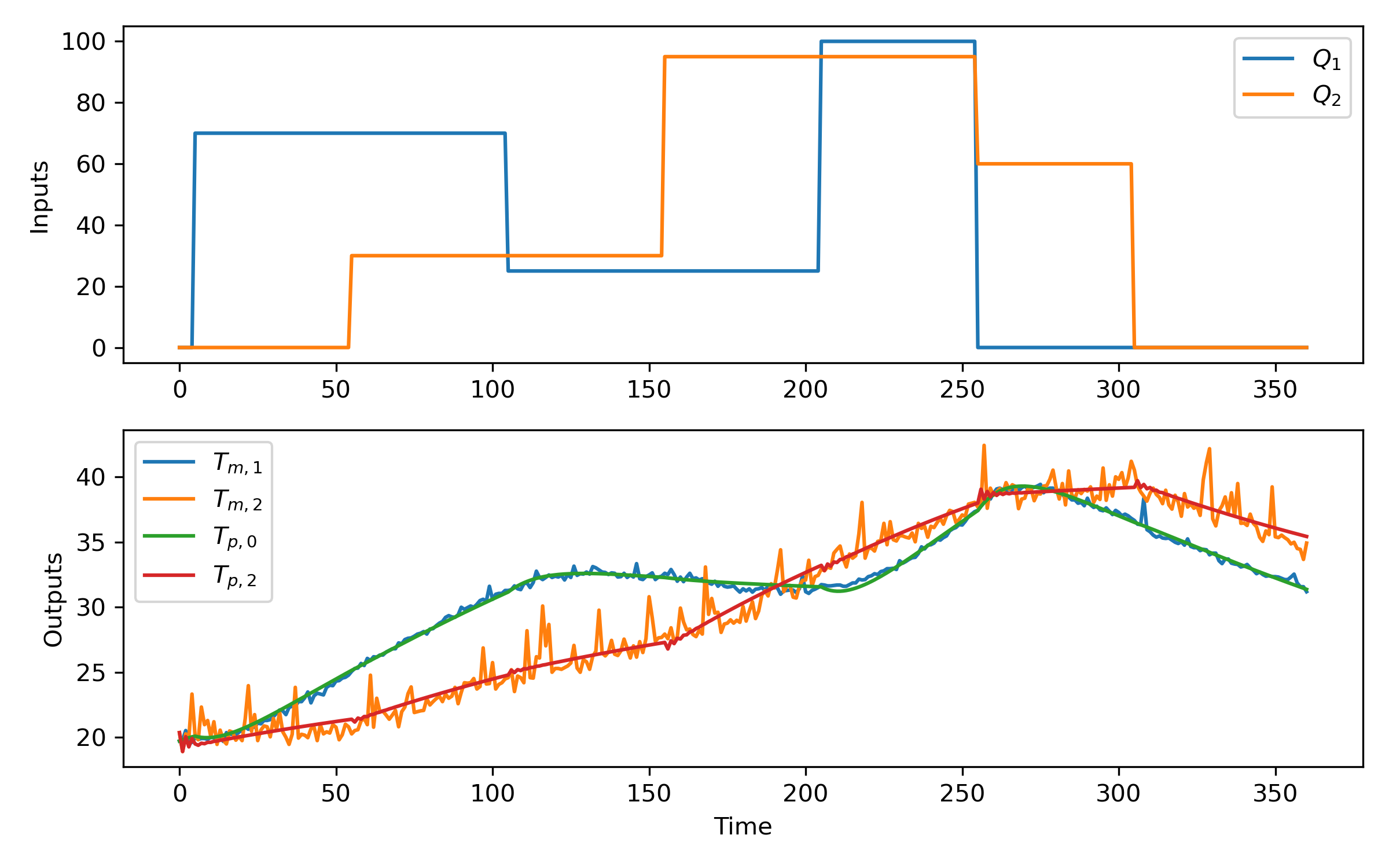
Step 1: Collect Data
import time
import pandas as pd
import matplotlib.pyplot as plt
x = {'Time':[],'Q1':[],'Q2':[],'T1':[],'T2':[]}
df = pd.DataFrame(x)
Q1 = 0; Q2 = 0
with tclab.TCLabModel() as lab:
for i in range(361):
Q1 = 70 if i==5 else Q1
Q1 = 25 if i==105 else Q1
Q1 = 100 if i==205 else Q1
Q1 = 0 if i>=255 else Q1
Q2 = 30 if i==55 else Q2
Q2 = 95 if i==155 else Q2
Q2 = 60 if i==225 else Q2
Q2 = 0 if i>=305 else Q2
lab.Q1(Q1); lab.Q2(Q2);
df.loc[i] = [i,Q1,Q2,lab.T1,lab.T2]
if i%10==0:
print(f'Q1:{Q1:5.2f} Q2:{Q2:5.2f} T1:{lab.T1:5.2f} T2:{lab.T2:5.2f}')
time.sleep(1)
df.set_index('Time',inplace=True)
print(df.describe())
df.to_csv('tclab2.csv')
df.plot(subplots=True)
plt.show()
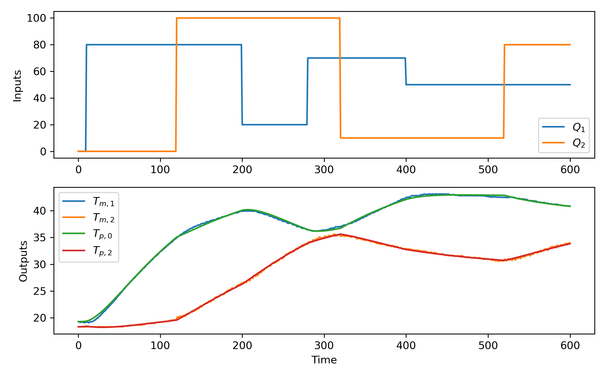
Step 2: System Identification with Q1 Steps or Q1 and Q2 Steps
import pandas as pd
import matplotlib.pyplot as plt
# load data and parse into columns
#url = 'tclab2.csv'
#url = 'http://apmonitor.com/dde/uploads/Main/tclab_step_test1.txt'
url = 'http://apmonitor.com/dde/uploads/Main/tclab_step_test2.txt'
data = pd.read_csv(url)
t = data['Time']
u = data[['Q1','Q2']]
y = data[['T1','T2']]
# generate time-series model
m = GEKKO(remote=False)
# system identification
na = 2 # output coefficients
nb = 2 # input coefficients
yp,p,K = m.sysid(t,u,y,na,nb)
plt.figure(figsize=(8,5))
plt.subplot(2,1,1)
plt.plot(t,u)
plt.legend([r'$Q_1$',r'$Q_2$'])
plt.ylabel('Inputs')
plt.subplot(2,1,2)
plt.plot(t,y)
plt.plot(t,yp)
plt.legend([r'$T_{m,1}$',r'$T_{m,2}$',r'$T_{p,0}$',r'$T_{p,2}$'])
plt.ylabel('Outputs')
plt.xlabel('Time')
plt.tight_layout()
plt.savefig('sysid.png',dpi=300)
plt.show()
✅ Knowledge Check
1. Which of the following statements accurately describes the ARX model?
- Incorrect. The ARX model combines both the autoregressive (AR) model and the exogenous input (X) model, taking into account both past values of the time series and external inputs.
- Correct. This is the essence of the ARX model where it combines the features of both the AR and X models.
- Incorrect. ARX time series models are linear representations of a dynamic system in discrete time.
- Incorrect. The ARX model accounts for both past values of the time series and past values of external input variables.
2. In the ARX model, what does the 'X' in ARX stand for?
- Incorrect. 'X' does not stand for Exponential in the context of the ARX model.
- Incorrect. 'X' does not stand for Exclusion in the context of the ARX model.
- Correct. In the ARX model, 'X' stands for Exogenous Input.
- Incorrect. 'X' does not stand for External Regression in the context of the ARX model.