Text Data Analysis

Importing and analyzing text data is common in data-driven engineering. Text files are often in the form of tables with a header row that describes each data column. Each row contains values as either numbers or strings that are separated by tabs, commas, or another type of delimiter. This tutorial is a demonstration of text data analysis with an application to vehicle performance analysis.

Import Libraries

Text files can be imported with the Python open() command, numpy.loadtxt() or pandas.read_csv(). The pandas library uses numpy as a base package and is a fully functional library for importing and analyzing data. This tutorial demonstrates the use of pandas for automotive data import and analysis.

import numpy as np
import pandas as pd
import matplotlib.pyplot as plt

[$[Get Code]]

Import Comma Separated Value (CSV) File

A 2021 Ford Explorer was driven and data recorded from the OBD-II port. The engine data was written to a CSV file and uploaded to the cloud for retrieval and analysis.

Auto_Ford2021.zip

The data file is stored in a zipped archive to compress the file for more efficient data storage and transfer. Pandas downloads and unzips the data file from the URL. The first two rows contain descriptive information about the data collection and are skipped with skiprows=2.

file = 'http://apmonitor.com/dde/uploads/Main/Auto_Ford2021.zip'
data = pd.read_csv(file,skiprows=2)

[$[Get Code]]

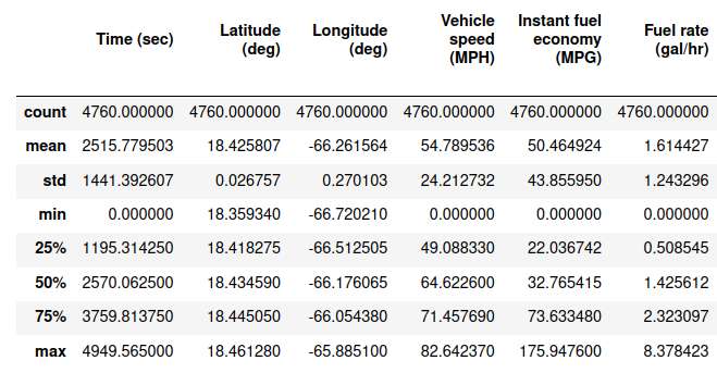
Summarize Data

Summary statistics provide insight, especially for large datasets. The count, mean, standard deviation, minimum, quartile, and maximum values are provided for each data column.

data.describe()

[$[Get Code]]

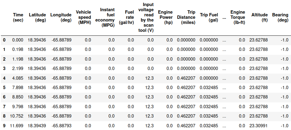
Display First 10 Rows

The first rows show that some of the sensors require 2-20 seconds to initialize. This creates data columns of 0 values or -1 values. For example, Bearing (deg) is 0-360° but is -1 initially until the sensor value is available. The data.head() function reports the first 5 rows by default. Other useful functions are data.tail() and data.sample() to report the end or randomly selected rows, respectively.

data.head(10)

[$[Get Code]]

Data Cleansing

It is important to remove bad data before analysis. Many machine learning methods are heavily influenced by outliers or bad data and may lead to the wrong conclusion. The first item is to remove a leading space in the column names.

# trim column names (extra leading space)
c = list(data.columns)
print('Before: ',c[0:3])
for i,ci in enumerate(c):
c[i] = ci.strip()
print('After: ',c[0:3])
data.columns = c

[$[Get Code]]

Conditional filters keep only those data rows that are True. The following data filter is to keep only the data rows with data['Bearing (deg)']>=0.

# filter data
# remove rows with Bearing (deg)=-1 (sensors are initializing)
data = data[data['Bearing (deg)']>=0]

[$[Get Code]]

In addition to removing the first rows as the data is initialized. It may be desirable to remove the last rows if the vehicle is stopped.

# remove data (remove last 5 rows)
data = data.iloc[:-5]

[$[Get Code]]

Data Reduction

Data reduction is important during data exploration phases for quick analysis and to resize the data set if only a subset is needed. The syntax data[::10] returns every 10th row from the original DataFrame.

# keep every 10th row
data = data[::10]

[$[Get Code]]

Set Time as Index

The table may have a key column that can be used to slice and reference the table by a unique row identifier. In this case, the Time (sec) is used as the DataFrame index.

# set time index
data.set_index('Time (sec)',inplace=True)

[$[Get Code]]

Add Column

Additional Series (columns) can be added to the DataFrame such as with custom calculations that are derived from other columns. In this case, the Average fuel economy (MPG) is calculated.

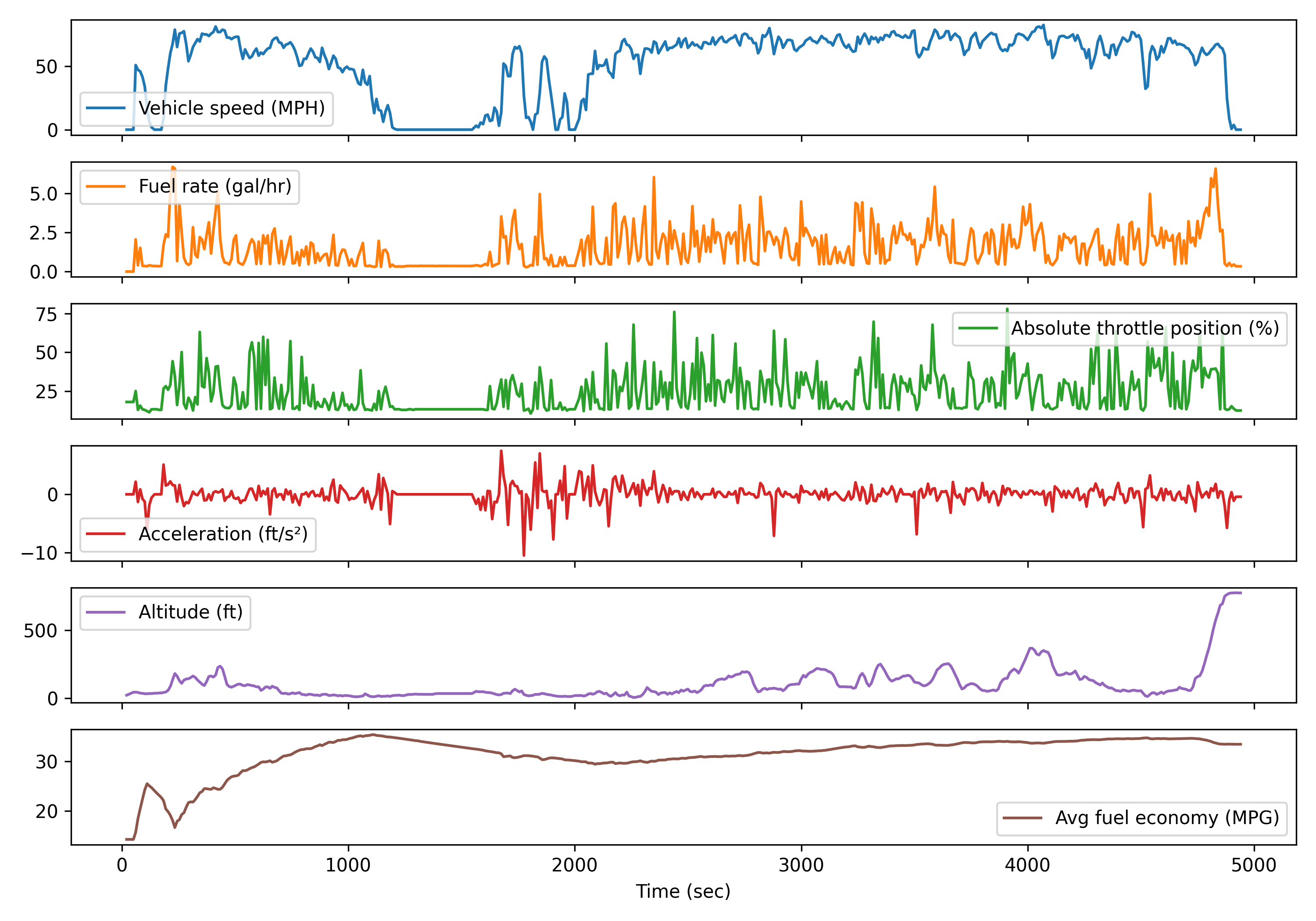
data['Avg fuel economy (MPG)'] = data['Trip Distance (miles)']/data['Trip Fuel (gal)']

[$[Get Code]]

Visualize Select Data

The data.plot() function creates a time series plot of the data. Adding subplot=True creates a separate plot for each trend. Only a subset of the data columns is included in the plot.

c = ['Vehicle speed (MPH)','Fuel rate (gal/hr)',
'Absolute throttle position (%)',
'Acceleration (ft/s²)','Altitude (ft)',
'Avg fuel economy (MPG)']
data[c].plot(figsize=(10,7),subplots=True)
plt.tight_layout()
plt.show()

[$[Get Code]]

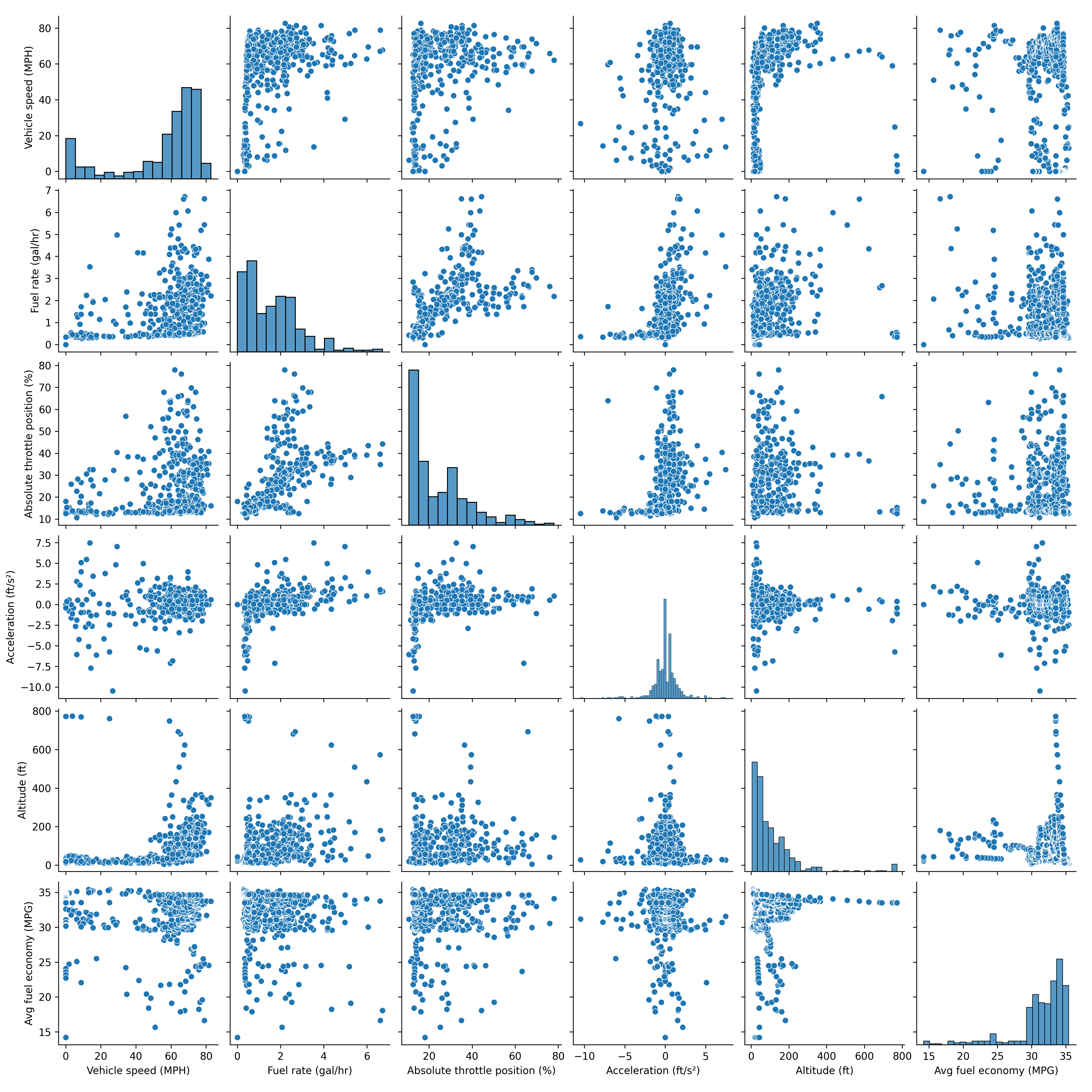
View Data Correlation

The Seaborn package creates custom visualizations from Pandas DataFrames. The sns.pairplot() is a scatter plot of each pair of data series in a matrix form. The plots on the diagonal show the distribution of that single variable and the off-diagonal plots show the correlation between data series.

import seaborn as sns
sns.pairplot(data[c])

[$[Get Code]]

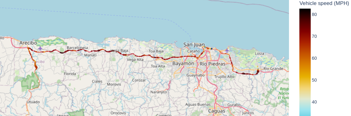
Display GPS Route

Plotly is a package for interactive data visualization. Install plotly with pip and restart the kernel, if not already installed.

#pip install plotly

[$[Get Code]]

A map box is created to show the vehicle route with color as the speed (MPH) and size of the dot as Fuel rate (gal/hr).

import plotly.express as px
fig = px.scatter_mapbox(data, lat="Latitude (deg)",\
lon="Longitude (deg)", \
color="Vehicle speed (MPH)", \
size="Fuel rate (gal/hr)", \
color_continuous_scale= \
px.colors.cyclical.IceFire, \
size_max=5, zoom=7)
fig.update_layout(
mapbox_style="open-street-map",
margin={"r": 0, "t": 0, "l": 0, "b": 0},
)
fig.show()

[$[Get Code]]

Export Modified Text File

data.to_csv('export_data.csv')

[$[Get Code]]

Activity

A 2021 Chrysler Pacifica is driven in Iowa. Compare the Ford Explorer and Chrysler Pacifica with the following:

Calculate average fuel economy for both vehicles
Include both vehicles on a pairplot
Create a map of the Chrysler Pacifica route

Auto_Chrysler2021.zip

file = 'http://apmonitor.com/dde/uploads/Main/Auto_Chrysler2021.zip'
dch = pd.read_csv(file,skiprows=2)

[$[Get Code]]

Solution

Python Text Data Solution |

Google Colab

# remove spaces from column names
c = list(dch.columns)
print('Before: ',c[0:3])
for i,ci in enumerate(c):
c[i] = ci.strip()
print('After: ',c[0:3])
dch.columns = c

# remove front rows where distance is zero
dch = dch[dch['Trip Distance (miles)']>1e-5]

# shift start time to zero
dch['Time (sec)'] = dch['Time (sec)'] - dch['Time (sec)'].iloc[0]

# filter based on
dch = dch[dch['Bearing (deg)']>=0]

# every 10th row
dch = dch[::10]

# set index
dch.set_index('Time (sec)',inplace=True)

# calculate avg fuel economy
a = dch['Trip Distance (miles)']
b = dch['Trip Fuel (gal)']
dch['Avg fuel economy (MPG)'] = a/b

t1 = np.array(data.index)/60
t2 = np.array(dch.index)/60
plt.figure(figsize=(10,8))
plt.subplot(4,1,1)
plt.plot(t1,data['Vehicle speed (MPH)'].values,'r-',label='Ford')
plt.plot(t2,dch['Vehicle speed (MPH)'].values,'b--',label='Chrysler')
plt.grid(); plt.ylabel('Speed (mph)')
plt.legend()

plt.subplot(4,1,2)
plt.plot(t1,data['Trip Distance (miles)'].values,'r-',label='Ford')
plt.plot(t2,dch['Trip Distance (miles)'].values,'b--',label='Chrysler')
plt.grid(); plt.ylabel('Distance (mi)')
plt.legend()

plt.subplot(4,1,3)
plt.plot(t1,data['Trip Fuel (gal)'].values,'r-',label='Ford')
plt.plot(t2,dch['Trip Fuel (gal)'].values,'b--',label='Chrysler')
plt.grid(); plt.ylabel('Trip Fuel (gal)')
plt.legend()

plt.subplot(4,1,4)
fmpg = str(round(data['Avg fuel economy (MPG)'].iloc[-1],1))
cmpg = str(round(dch['Avg fuel economy (MPG)'].iloc[-1],1))
plt.plot(t1,data['Avg fuel economy (MPG)'].values,'r-', \
label='Ford MPG: '+fmpg)
plt.plot(t2,dch['Avg fuel economy (MPG)'].values,'b--', \
label='Chrysler MPG: '+cmpg)
plt.grid(); plt.ylabel('Fuel Economy (MPG)')
plt.xlabel('Time (min)'); plt.legend()
plt.show()

# generate pairplot
c = ['Vehicle speed (MPH)','Fuel rate (gal/hr)',
'Absolute throttle position (%)',
'Acceleration (ft/s²)','Avg fuel economy (MPG)','Vehicle']
# add vehicle specification
data['Vehicle'] = 'Ford'
dch['Vehicle'] = 'Chrysler'

c1 = data[c].copy()
c2 = dch[c].copy()
c = pd.concat((c1,c2)).reset_index(drop=True)
sns.pairplot(c,hue='Vehicle')
plt.show()

# generate map
import plotly.express as px
color = px.colors.cyclical.IceFire
fig = px.scatter_mapbox(dch, lat="Latitude (deg)", \
lon="Longitude (deg)", \
color="Vehicle speed (MPH)", \
size="Fuel rate (gal/hr)", \
color_continuous_scale=color, \
size_max=5, zoom=7)
fig.update_layout(
mapbox_style="open-street-map",
margin={"r": 0, "t": 0, "l": 0, "b": 0},
)
fig.show()

[$[Get Code]]

Additional Data

Auto_Mazda2023a.zip

Auto_Mazda2023b.zip

✅ Knowledge Check

1. To import text data from a CSV file, which library and function is recommended?

A. Python open() command

Incorrect. While the Python open() command can be used to open text files, it is not specifically designed for CSV files, which may contain structured data.

B. numpy.loadtxt()

Incorrect. numpy.loadtxt() is a function to load data from a text file. However, for structured CSV files, pandas.read_csv() is more suitable due to its flexibility and data handling capabilities.

C. pandas.read_csv()

Correct. pandas.read_csv() is specifically designed to import structured data from CSV files, making it an excellent choice for this task.

D. matplotlib.pyplot

Incorrect. matplotlib.pyplot is used for plotting and visualization, not for importing text data.

2. After importing data, what is the primary reason to perform data cleansing?

A. To add new columns to the data

Incorrect. Adding new columns is not specifically related to data cleansing. Data cleansing primarily focuses on improving the quality and reliability of the data.

B. To change the visual representation of the data

Incorrect. Data visualization comes after the data has been cleansed and processed, and is not the primary reason for data cleansing.

C. To remove outliers or bad data

Correct. One of the primary reasons for data cleansing is to remove outliers, bad data, or any inconsistencies that might affect the subsequent analysis.

D. To reduce the size of the dataset for faster processing

Incorrect. Data reduction or sampling is a technique to decrease the size of the dataset. While this might be a subsequent step after data cleansing, it is not the primary reason for data cleansing.

Data-Driven Engineering