Automation with LSTM Network
The purpose of this exercise is to automate a temperature control process with an LSTM network. The LSTM network is trained from a PID (Proportional Integral Derivative) controller or a Model Predictive Controller (MPC). LSTM (Long Short Term Memory) networks are a special type of RNN (Recurrent Neural Network) that is structured to remember and predict based on long-term dependencies that are trained with time-series data. An LSTM repeating module has four interacting components.
The LSTM is trained (parameters adjusted) with an input window of prior data and minimized difference between the predicted and next measured value. Sequential methods predict just one next value based on the window of prior data. In this case, the error between the set point and measured value is the feature and the heater value is the output label.



Background: Proportional Integral Derivative (PID) control automatically adjusts a control output based on the difference between a set point (SP) and a measured process variable (PV). The value of the controller output `u(t)` is transferred as the system input.
$$e(t) = SP-PV$$
$$u(t) = u_{bias} + K_c \, e(t) + \frac{K_c}{\tau_I}\int_0^t e(t)dt - K_c \tau_D \frac{d(PV)}{dt}$$
The `u_{bias}` term is a constant that is typically set to the value of `u(t)` when the controller is first switched from manual to automatic mode. The three tuning values for a PID controller are the controller gain, `K_c`, the integral time constant `\tau_I`, and the derivative time constant `\tau_D`. The value of `K_c` is a multiplier on the proportional error and integral term and a higher value makes the controller more aggressive at responding to errors away from the set point. The integral time constant `\tau_I` (also known as integral reset time) must be positive and has units of time. As `\tau_I` gets smaller, the integral term is larger because `\tau_I` is in the denominator. Derivative time constant `\tau_D` also has units of time and must be positive. The set point (SP) is the target value and process variable (PV) is the measured value that may deviate from the desired value. The error from the set point is the difference between the SP and PV and is defined as `e(t) = SP - PV`.
Objective: Train and deploy an LSTM network to adjust the heater (Q) to regulate the TCLab temperature to a requested set point. Submit source code and a summary memo (max 2 pages) of your results.
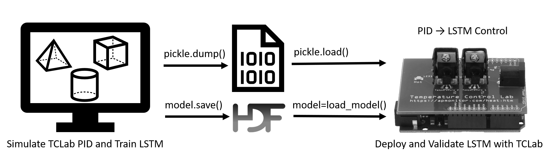
Replace the PID control with the LSTM network. Store the LSTM network from the Jupyter notebook to deploy the machine learned model.
import time
import numpy as np
from simple_pid import PID
import matplotlib.pyplot as plt
# Create PID controller
pid = PID(Kp=5.0,Ki=0.05,Kd=1.0,\
setpoint=50,sample_time=1.0,\
output_limits=(0,100))
n = 300
tm = np.linspace(0,n-1,n)
T1 = np.zeros(n); Q1 = np.zeros(n)
lab = tclab.TCLab()
for i in range(n):
# read temperature
T1[i] = lab.T1
# PID control
Q1[i] = pid(T1[i])
lab.Q1(Q1[i])
if i%50==0:
print('Time OP PV SP')
if i%5==0:
print(i,round(Q1[i],2), T1[i], pid.setpoint)
# wait sample time
time.sleep(pid.sample_time) # wait 1 sec
lab.close()
After the controller completes the 5 minute test, generate a figure of the response with the temperature (T1), temperature target set point (TSP), and heater (Q1).
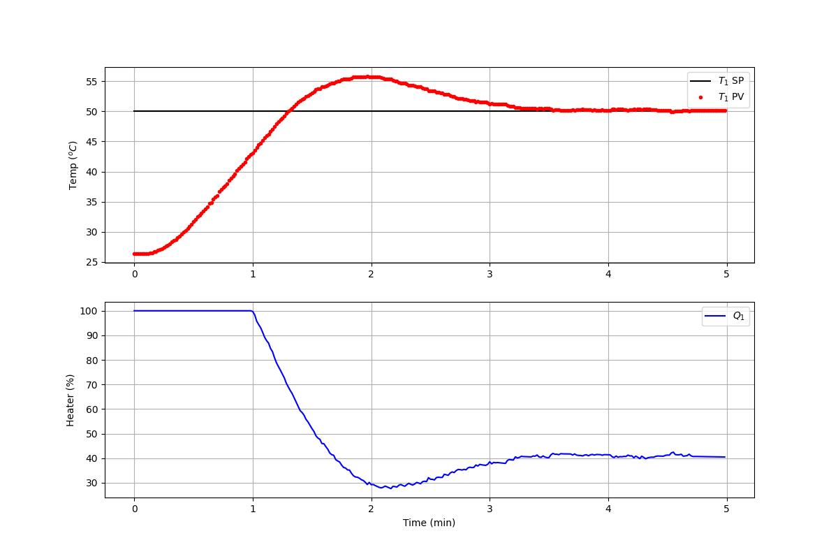
plt.figure(figsize=(12,8))
plt.subplot(2,1,1)
plt.grid()
plt.plot([0,tm[-1]/60.0],[50,50],'k-',label=r'$T_1$ SP')
plt.plot(tm/60.0,T1,'r.',label=r'$T_1$ PV')
plt.ylabel(r'Temp ($^oC$)')
plt.legend()
plt.subplot(2,1,2)
plt.grid()
plt.plot(tm/60.0,Q1,'b-',label=r'$Q_1$')
plt.ylabel(r'Heater (%)'); plt.xlabel('Time (min)')
plt.legend()
plt.show()
LSTM Emulates SISO MPC
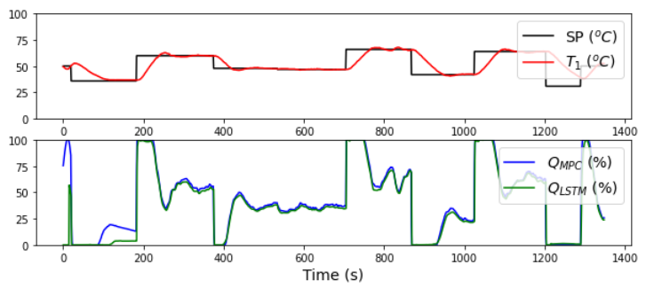
The LSTM Network learns from any type of sequence, not just PID control. The PID controller is replaced with a Single Input (Q1), Single Output (T1) Model Predictive Controller (MPC). The LSTM Network learns the MPC response, similar to the PID controller.
An extension of this work is to train from a multivariate controller with Multiple Inputs (Q1, Q2), Multiple Outputs (T1, T2). The LSTM Network inputs and outputs can be adapted to accommodate the increased dimensions. See LSTM Networks in the Dynamic Optimization course for training an LSTM from a MIMO (2x2) MPC.
Solution Help
The challenge for both the PID and SISO MPC case studies is to deploy the LSTM controller, independent of any training program. The training can occur offline while the online implementation is deployed to a SCADA (Scheduling and Data Acquisition) system such as a Distributed Control System (DCS) or Programmable Logic Controller (PLC). Below is sample code for deploying the saved data in lstm_control.pkl and LSTM network model in lstm_control.h5. Update the cycle time (sleep time) to 1 sec for PID control and 2 sec for MPC. To test this code, either use the device with TCLab() or switch to the digital twin with TCLabModel().

import time
import numpy as np
import matplotlib.pyplot as plt
import pickle
from keras.models import load_model
# PID: 1 sec, MPC: 2 sec
cycle_time = 2
tclab_hardware = False # switch to True if hardware available
h5_file,s_x,s_y,window = pickle.load(open('lstm_control.pkl','rb'))
model = load_model(h5_file)
if tclab_hardware:
mlab = tclab.TCLab # Physical hardware
else:
mlab = tclab.setup(connected=False,speedup=10) # Emulator
def lstm(T1_m, Tsp_m):
# Calculate error (necessary feature for LSTM input)
err = Tsp_m - T1_m
# Format data for LSTM input
X = np.vstack((Tsp_m,err)).T
Xs = s_x.transform(X)
Xs = np.reshape(Xs, (1, Xs.shape[0], Xs.shape[1]))
# Predict Q for controller and unscale
Q1c_s = model.predict(Xs)
Q1c = s_y.inverse_transform(Q1c_s)[0][0]
# Ensure Q1c is between 0 and 100
Q1c = np.clip(Q1c,0.0,100.0)
return Q1c
tf = 300 # final time (sec)
n = int(tf/cycle_time) # cycles
tm=[]; T1=[]; Q1=[] # storage
lab = mlab()
i = 0
for t in tclab.clock(tf, cycle_time):
# record time
tm.append(t)
# read temperature
T1.append(lab.T1)
# LSTM control
if i>=window:
T1_m = T1[i-window:i]
else:
insert = np.ones(window-i)*T1[0]
T1_m = np.concatenate((insert,T1[0:-1]))
Tsp_m = 50*np.ones(window)
Q1.append(lstm(T1_m,Tsp_m)); lab.Q1(Q1[-1])
if i%50==0:
print('Time Q1 T1 SP')
if i%5==0:
print("{0:4d} {1:6.2f} {2:6.2f} {3:4d}"\
.format(i,Q1[-1],T1[-1],50))
i+=1
lab.close()
# Create Figure
tmin = np.array(tm)/60.0
plt.figure(figsize=(10,6))
plt.subplot(2,1,1)
plt.grid()
plt.plot([0,0.01,1,tmin[-1]],[T1[0],50,50,50],\
'k-',label=r'$T_1$ SP')
plt.plot(tmin,T1,'r.',label=r'$T_1$ PV')
plt.ylabel(r'Temp ($^oC$)')
plt.legend()
plt.subplot(2,1,2)
plt.grid()
plt.plot(tmin,Q1,'b-',label=r'$Q_1$')
plt.ylabel(r'Heater (%)'); plt.xlabel('Time (min)')
plt.legend()
plt.show()
References
- Lewis, N., PID Control Emulation with LSTM Network, Part 1, Part 2, Part 3, Part 4, Towards Data Science, 2020.
- Phi, M., Illustrated Guide to LSTM’s and GRU’s: A step by step explanation, Towards Data Science, Sept 2018.
- See Deploy Machine Learning and LSTM Networks in Machine Learning for Engineers (this course) and LSTM Network Replaces MIMO (2x2) MPC in the Dynamic Optimization course.
Generative AI Learning
Use these prompts to test your understanding after completing the exercise. Direct the AI — you own the training data and the hardware test.
Tip: The honest comparison is closed-loop, on hardware, same setpoint sequence: PID vs LSTM. Training-set prediction accuracy is NOT controller performance — a network can fit the PID's output to 1% and still fail in closed loop, because its own small errors feed back into its next input.
What to Turn In
Submit your source code and a summary memo (PDF, maximum 2 pages) that curates your results into a demonstration of what you learned. You may use Generative AI to help write the memo, but you must guide it to the correct visualizations, justifications, and assumptions. Answer these questions:
- Describe the training data: which controller generated it (PID or MPC), the setpoint sequence, and why it covers the deployment range. Include the training/validation loss curves.
- Show the closed-loop comparison on the TCLab: temperature and heater plots for PID and for the LSTM over the same setpoint schedule, with tracking error quantified for both.
- Report one break-it test: the plot, what the LSTM commanded, and your diagnosis of why.
- When is a learned controller an acceptable replacement for the PID it imitated, and what safeguard (output clipping, fallback controller, out-of-range watchdog) would you require before trusting it unattended? Answer from your own test evidence.