Gaussian Process Regression
Gaussian process (GP) regression is a type of probabilistic model that can be used for regression tasks. It is a non-parametric method that is based on the assumption that the function to be learned is drawn from a Gaussian process. This assumption allows the model to make predictions with a well-defined uncertainty, which can be useful for tasks such as active learning and uncertainty-aware decision making.
Mathematically, the GP regression model can be written as follows. Let `x_1, x_2,\ldots, x_n` be the input data points, where `x_i \in \mathbb{R}^d` is a d-dimensional vector. Let `y_1, y_2,\ldots, y_n` be the corresponding output values, where `y_i \in \mathbb{R}` is a scalar. The GP regression model assumes that the function f that relates the inputs to the outputs is drawn from a Gaussian process with mean function `\mu` and covariance function k. The distribution of f at a set of test points x* is then given by:
$$f(x^*) \sim \mathcal{N}(\mu(x^*), k(x^*, x^*))$$
The mean function and covariance function are typically defined using kernel functions. For example, the commonly used squared exponential kernel is defined as:
$$k(x_i, x_j) = \exp \left( -\frac{1}{2} ||x_i - x_j||^2 \right)$$
Given a set of training data (x, y), the GP regression model uses Bayesian inference to learn the distribution of f that is most likely to have generated the data. This involves computing the posterior distribution of f given the data, which is defined as:
$$p(f|x, y) = \frac{p(y|x,f) p(f)}{p(y|x)}$$
where (y|x,f) is the likelihood of the data given the function f, p(f) is the prior distribution of f, and p(y|x) is the marginal likelihood of the data.
Once the posterior distribution of f has been learned, the model can make predictions at new test points x* by computing the posterior predictive distribution, which is defined as:
$$p(f^*|x^*, y, x) = \int p(f^*|x^*,f) p(f|y,x) df$$
This distribution provides a measure of the uncertainty of the prediction, which can be useful for tasks such as active learning and uncertainty-aware decision making.
Gaussian process regression (GPR) uses training data, similar to k-Nearest Neighbors, to make predictions. It works well with small data sets and provides a prediction with uncertainty quantification.
The prior mean and prior covariance must be specified. The covariance is specified as a kernel object. The kernel hyper-parameters are optimized during fitting by maximizing the log-marginal-likelihood (LML) based on the specified optimizer. This maximization is a non-convex optimization (multiple local optima) so the optimizer is restarted multiple times. The first iteration starts from the initial hyper-parameters and subsequent iterations use randomly selected hyper-parameters within the allowed range.
Advantages: Predictions are an interpolation of the training data for regular kernels. The predictions also produce a probability for a confidence interval. GP can use many different kernels or use the default standard kernels.
Disadvantages: GP is not efficient when the number of features is greater than ~30. GP is not sparse with all of the features and samples used to perform the prediction.
| Hyperparameter | Description | Typical range/values |
|---|---|---|
kernel |
Kernel specifying covariance function of the GP (e.g., RBF, Matern). | Composite kernels combining RBF, WhiteNoise, etc.; start with RBF |
length_scale |
Length scale of the RBF kernel; controls the smoothness of the function. | 0.01 – 100 (logarithmic range) |
alpha |
Value added to the diagonal of the kernel matrix during fitting; acts as the noise level. | 0.0 – 0.5 (set to noise variance; e.g., 0.75²) |
n_restarts_optimizer |
Number of times the optimizer is restarted to find a better parameter set. | 0 – 10 |
kernel = gp.kernels.ConstantKernel(1.0, (1e-1, 1e3)) * \
gp.kernels.RBF(10.0, (1e-3, 1e3))
# Prior mean constant and zero (normalize_y=False)
# Prior mean from the data mean (normalize_y=True)
s = gp.GaussianProcessRegressor(kernel=kernel,\
n_restarts_optimizer=10,\
alpha=0.1,\
normalize_y=True)
s.fit(XA,yA)
yP,stdev = s.predict(XB, return_std=True)
Sample Code with Data
import matplotlib.pyplot as plt
import sklearn.gaussian_process as gp
# Gaussian Process Regression
kernel = gp.kernels.ConstantKernel(1.0, (1e-1, 1e3)) * \
gp.kernels.RBF(10.0, (1e-3, 1e3))
s = gp.GaussianProcessRegressor(kernel=kernel,\
n_restarts_optimizer=10,\
alpha=0.1,\
normalize_y=True)
# Training Data
XA = np.array([4,5,2,3,-1,1,6,7])
yA = np.array([0.3,0.8,-0.05,0.1,-0.8,-0.5,0.5,0.65])
s.fit(XA.reshape(-1,1),yA)
# Test data
XB = np.array([4.5,5.5,2.5,3.5,-1.5,1.5,5.9,7.8])
yB = np.array([0.35,0.75,-0.06,0.13,-0.85,-0.45,0.58,0.69])
yP,stdev = s.predict(XB.reshape(-1,1), return_std=True)
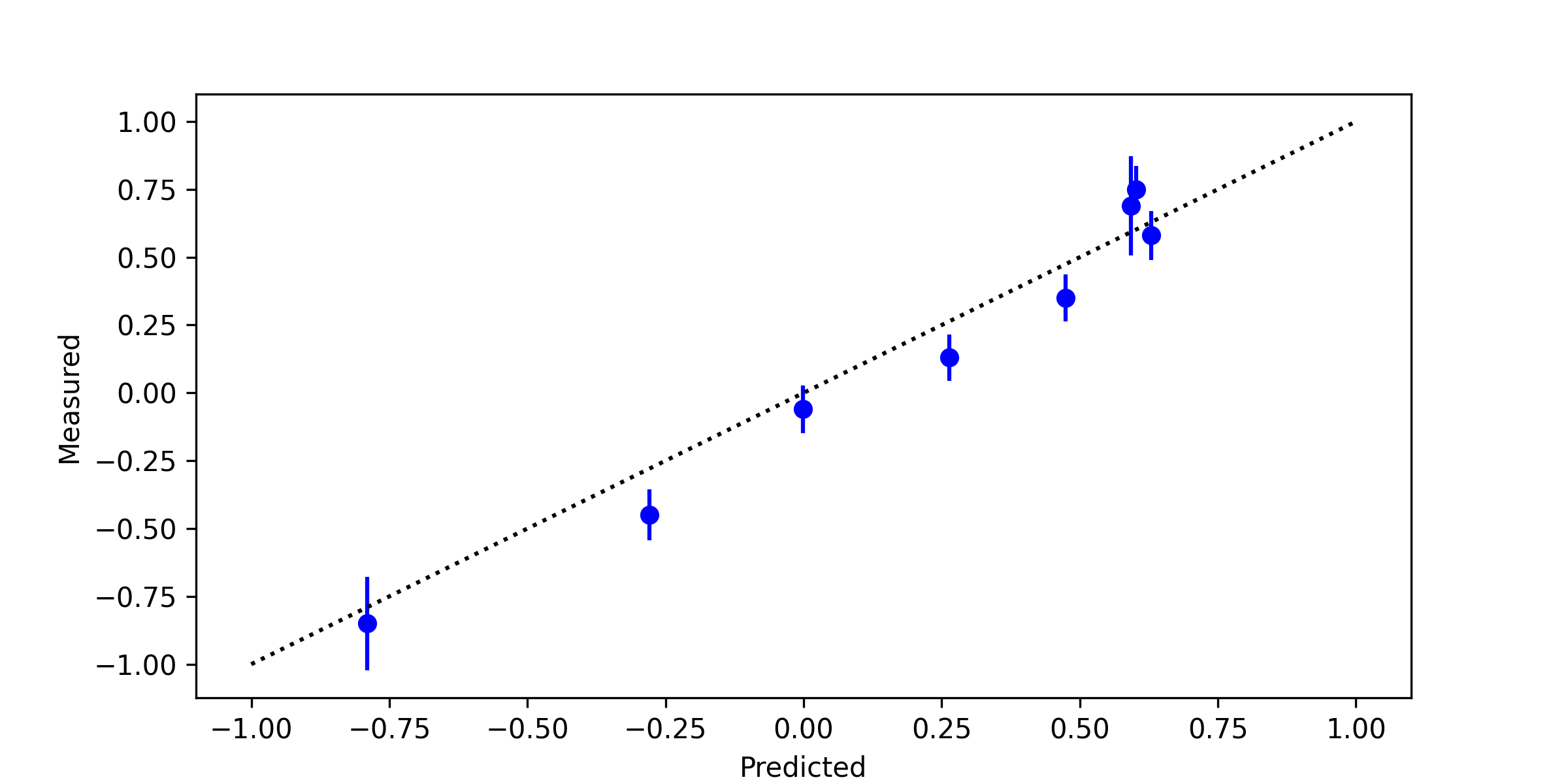
# Plot results
plt.figure(figsize=(8,4))
plt.plot([-1,1],[-1,1],'k:')
plt.errorbar(yP,yB,stdev,linestyle='None',
marker='o',color='blue')
plt.xlabel('Predicted')
plt.ylabel('Measured')
plt.savefig('gpr.png',dpi=300)
plt.show()
MATLAB Live Script

References
- Gaussian Processes, Scikit-learn at https://scikit-learn.org/stable/modules/gaussian_process.html
- Sit, H., Quick Start to Gaussian Process Regression: A quick guide to understanding Gaussian process regression (GPR) and using scikit-learn’s GPR package, Towards Data Science, Published: Jun 19, 2019.