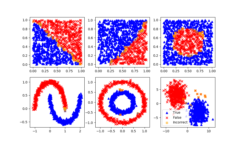
Decision Tree
A decision tree classifier is a type of machine learning algorithm that is used to predict the class or label of an input data point by making decisions based on the values of the features of the data.
Given attribute data (features) together with its classes (labels), a decision tree produces a sequence of rules that can be used to classify the data. The algorithm works by recursively partitioning the training data into smaller subsets based on the values of the features, until each subset contains only data points belonging to a single class. The resulting tree structure is then used to make predictions on new data points by traversing the tree and making decisions at each node based on the values of the input data point's features.
Advantages: Decision Tree is simple to understand and visualise, requires little data preparation, and can handle both numerical and categorical data.
Disadvantages: Decision tree can create complex trees that do not generalise well, and decision trees can be unstable because small variations in the data might result in a completely different tree being generated.
| Hyperparameter | Description | Typical range/values |
|---|---|---|
max_depth |
Maximum depth of the tree. Smaller values restrict complexity and help prevent overfitting; unlimited depth can overfit. | 1 – 20 |
min_samples_split |
Minimum number of samples required to split an internal node. | 2 – 20 |
min_samples_leaf |
Minimum number of samples required to be at a leaf node. | 1 – 20 |
max_features |
Number of features to consider when looking for the best split; controls randomness in splits. | ‘auto’ (all), ‘sqrt’, ‘log2’ or float fraction |
criterion |
Function used to measure the quality of a split. | ‘gini’, ‘entropy’ |
splitter |
Strategy used to choose the split at each node. | ‘best’, ‘random’ |
min_weight_fraction_leaf |
Minimum weighted fraction of the sum total of weights (of all the input samples) required to be at a leaf node. | 0.0 – 0.2 |
Decision Tree in Python
# Create a decision tree classifier
model = DecisionTreeClassifier()
# Train the model on the training data
model.fit(X_train, y_train)
# Make predictions on the test set
y_pred = model.predict(X_test)
In this example, we first create a decision tree classifier using the DecisionTreeClassifier class from scikit-learn. Then, we train the model on the training data using the fit method. Finally, we use the trained model to make predictions on the test set using the predict method. There are additional options such as max_depth to tune the performance of the decision tree.
dtree = DecisionTreeClassifier(max_depth=10,random_state=101,\
max_features=None,min_samples_leaf=5)
dtree.fit(XA,yA)
yP = dtree.predict(XB)

Optical Character Recognition with Decision Tree Example

Optical character recognition (OCR) is the process of extracting text from images or scanned documents. OCR algorithms are typically based on machine learning models that are trained on large datasets of images containing text. Here is an example of OCR using a decision tree classifier in Python using the scikit-learn library:
from sklearn.datasets import load_digits
from sklearn.tree import DecisionTreeClassifier
from sklearn.model_selection import train_test_split
# Load the dataset of images of handwritten digits
digits = load_digits()
# Split the dataset into training and testing sets
X_train, X_test, y_train, y_test = train_test_split(digits.data,
digits.target,
random_state=0)
# Create a decision tree classifier
model = DecisionTreeClassifier()
# Train the model using the training set
model.fit(X_train, y_train)
# Evaluate the model performance on the test set
accuracy = model.score(X_test, y_test)
print("Accuracy: %0.2f" % accuracy)
In this example, we first load the digits dataset from scikit-learn, which contains images of handwritten digits. Then, we create a decision tree classifier using the DecisionTreeClassifier class. Next, we train the model on the digits dataset. Finally, we use the trained model to make predictions on new images to generate an accuracy score.
Note that this is just a simple example of OCR using a decision tree classifier in scikit-learn, and many other more advanced OCR algorithms and libraries exist. Decision tree classifiers may not be the most effective model for OCR tasks, as they are not well-suited to high-dimensional datasets like images.
Below is a more complete example with a train / test data split.
from sklearn.model_selection import train_test_split
import matplotlib.pyplot as plt
import numpy as np
from sklearn.tree import DecisionTreeClassifier
classifier = DecisionTreeClassifier(max_depth=10,random_state=101,\
max_features=None,min_samples_leaf=5)
# The digits dataset
digits = datasets.load_digits()
n_samples = len(digits.images)
data = digits.images.reshape((n_samples, -1))
# Split into train and test subsets (50% each)
X_train, X_test, y_train, y_test = train_test_split(
data, digits.target, test_size=0.5, shuffle=False)
# Learn the digits on the first half of the digits
classifier.fit(X_train, y_train)
# Test on second half of data
n = np.random.randint(int(n_samples/2),n_samples)
print('Predicted: ' + str(classifier.predict(digits.data[n:n+1])[0]))
# Show number
plt.imshow(digits.images[n], cmap=plt.cm.gray_r, interpolation='nearest')
plt.show()
Further Reading
- Brownlee, J. How To Implement The Decision Tree Algorithm From Scratch In Python, Machine Learning Mastery, Nov 2016.
def test_split(index, value, dataset):
left, right = list(), list()
for row in dataset:
if row[index] < value:
left.append(row)
else:
right.append(row)
return left, right
# Calculate the Gini index for a split dataset
def gini_index(groups, classes):
# count all samples at split point
n_instances = float(sum([len(group) for group in groups]))
# sum weighted Gini index for each group
gini = 0.0
for group in groups:
size = float(len(group))
# avoid divide by zero
if size == 0:
continue
score = 0.0
# score the group based on the score for each class
for class_val in classes:
p = [row[-1] for row in group].count(class_val) / size
score += p * p
# weight the group score by its relative size
gini += (1.0 - score) * (size / n_instances)
return gini
# Select the best split point for a dataset
def get_split(dataset):
class_values = list(set(row[-1] for row in dataset))
b_index, b_value, b_score, b_groups = 999, 999, 999, None
for index in range(len(dataset[0])-1):
for row in dataset:
groups = test_split(index, row[index], dataset)
gini = gini_index(groups, class_values)
if gini < b_score:
b_index, b_value, b_score, b_groups = index, row[index], gini, groups
return {'index':b_index, 'value':b_value, 'groups':b_groups}
# Create a terminal node value
def to_terminal(group):
outcomes = [row[-1] for row in group]
return max(set(outcomes), key=outcomes.count)
# Create child splits for a node or make terminal
def split(node, max_depth, min_size, depth):
left, right = node['groups']
del(node['groups'])
# check for a no split
if not left or not right:
node['left'] = node['right'] = to_terminal(left + right)
return
# check for max depth
if depth >= max_depth:
node['left'], node['right'] = to_terminal(left), to_terminal(right)
return
# process left child
if len(left) <= min_size:
node['left'] = to_terminal(left)
else:
node['left'] = get_split(left)
split(node['left'], max_depth, min_size, depth+1)
# process right child
if len(right) <= min_size:
node['right'] = to_terminal(right)
else:
node['right'] = get_split(right)
split(node['right'], max_depth, min_size, depth+1)
# Build a decision tree
def build_tree(train, max_depth, min_size):
root = get_split(train)
split(root, max_depth, min_size, 1)
return root
# Print a decision tree
def print_tree(node, depth=0):
if isinstance(node, dict):
print('%s[X%d < %.3f]' % ((depth*' ', (node['index']+1), node['value'])))
print_tree(node['left'], depth+1)
print_tree(node['right'], depth+1)
else:
print('%s[%s]' % ((depth*' ', node)))
dataset = [[2.771244718,1.784783929,0],
[1.728571309,1.169761413,0],
[3.678319846,2.81281357,0],
[3.961043357,2.61995032,0],
[2.999208922,2.209014212,0],
[7.497545867,3.162953546,1],
[9.00220326,3.339047188,1],
[7.444542326,0.476683375,1],
[10.12493903,3.234550982,1],
[6.642287351,3.319983761,1]]
tree = build_tree(dataset, 1, 1)
print_tree(tree)
def predict(node, row):
if row[node['index']] < node['value']:
if isinstance(node['left'], dict):
return predict(node['left'], row)
else:
return node['left']
else:
if isinstance(node['right'], dict):
return predict(node['right'], row)
else:
return node['right']
# predict with a stump
stump = {'index': 0, 'right': 1, 'value': 6.642287351, 'left': 0}
for row in dataset:
prediction = predict(stump, row)
print('Expected=%d, Got=%d' % (row[-1], prediction))
  Expected=0, Got=0
  Expected=0, Got=0
  Expected=0, Got=0
  Expected=0, Got=0
  Expected=0, Got=0
  Expected=1, Got=1
  Expected=1, Got=1
  Expected=1, Got=1
  Expected=1, Got=1
  Expected=1, Got=1
✅ Knowledge Check
1. Why is the Decision Tree a popular classifier, especially for beginners in machine learning?
- Incorrect. Decision trees do not necessarily require large amounts of data. Their popularity is due to their simplicity and ease of visualization.
- Incorrect. Decision trees are not particularly well-suited to high-dimensional datasets like images. They are popular because they are easy to understand and visualize.
- Correct. Decision trees are indeed popular due to their simplicity, visualization capabilities, and minimal data preparation requirements.
- Incorrect. Decision trees do not always provide the most accurate predictions, especially if they overfit to the training data. Their advantage lies in their interpretability and visualization.
2. What is a potential disadvantage of using Decision Trees?
- Incorrect. Decision trees can handle both numerical and categorical data.
- Correct. Decision trees can overfit to the training data, resulting in complex trees that perform poorly on unseen data.
- Incorrect. Decision trees can be used for both classification and regression tasks.
- Incorrect. Decision trees can handle both numerical and categorical data.
Return to Classification Overview


