TCLab D - Empirical Model Estimation
Main.TCLabD History
Show minor edits - Show changes to markup
Virtual TCLab on Google Colab
plt.show() (:sourceend:) (:divend:)
(:toggle hide gekko_labDARX button show="Lab D: Python GEKKO 2nd Order ARX":) (:div id=gekko_labDARX:) (:source lang=python:) from gekko import GEKKO import numpy as np import pandas as pd import matplotlib.pyplot as plt
- load data and parse into columns
url = 'http://apmonitor.com/do/uploads/Main/tclab_dyn_data2.txt' data = pd.read_csv(url) t = data['Time'] u = data'H1','H2'? y = data'T1','T2'?
m = GEKKO()
- system identification
na = 2 # output coefficients nb = 2 # input coefficients yp,p,K = m.sysid(t,u,y,na,nb,pred='meas')
plt.figure() plt.subplot(2,1,1) plt.plot(t,u,label=r'$Heater_1$') plt.legend([r'$Heater_1$',r'$Heater_2$']) plt.ylabel('Heaters') plt.subplot(2,1,2) plt.plot(t,y) plt.plot(t,yp,) plt.legend([r'$T1_{meas}$',r'$T2_{meas}$', r'$T1_{pred}$',r'$T2_{pred}$']) plt.ylabel('Temperature (°C)') plt.xlabel('Time (sec)')
See information on Second Order Systems and Moving Horizon Estimation.
See information on Second Order Systems and Moving Horizon Estimation.
- Solution in Python and MATLAB
<iframe width="560" height="315" src="https://www.youtube.com/embed/Cp6fPUptc74" frameborder="0" allow="accelerometer; autoplay; encrypted-media; gyroscope; picture-in-picture" allowfullscreen></iframe>
<iframe width="560" height="315" src="https://www.youtube.com/embed/yRvffV7ZPOA" frameborder="0" allow="accelerometer; autoplay; encrypted-media; gyroscope; picture-in-picture" allowfullscreen></iframe>
(:html:) <iframe width="560" height="315" src="https://www.youtube.com/embed/Cp6fPUptc74" frameborder="0" allow="accelerometer; autoplay; encrypted-media; gyroscope; picture-in-picture" allowfullscreen></iframe> (:htmlend:)
        plt.plot(tm[0:i],tau3s[0:i]*10,'r--',label=r'$\tau_3$ x 10')
        plt.ylabel('Gains')
        plt.plot(tm[0:i],tau3s[0:i]*10,'r--',label=r'$\tau_3$ x 10')
        plt.ylabel('Time constant')
(:sourceend:) (:divend:)
2nd Order System Identification with MHE
See information on Second Order Systems and Moving Horizon Estimation.
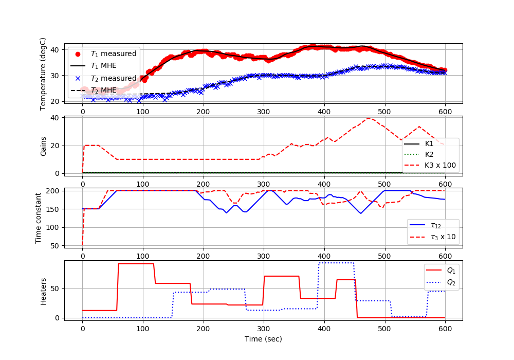
(:toggle hide gekko_labDMHE button show="Lab D: Python GEKKO 2nd Order MHE":) (:div id=gekko_labDMHE:) (:source lang=python:) import numpy as np import time import matplotlib.pyplot as plt import random
- get gekko package with:
- pip install gekko
from gekko import GEKKO
- get tclab package with:
- pip install tclab
from tclab import TCLab
- save txt file
def save_txt(t,Q1,Q2,T1,T2):
    data = np.vstack((t,Q1,Q2,T1,T2))  # vertical stack
    data = data.T                 # transpose data
    top = 'Time (sec), Heater 1, Heater 2, '         + 'Temperature 1, Temperature 2'
    np.savetxt('data.txt',data,delimiter=',',header=top,comments='')
- Connect to Arduino
a = TCLab()
- Final time
tf = 10 # min
- number of data points (every 3 seconds)
n = tf * 20 + 1
- Configure heater levels
- Percent Heater (0-100%)
Q1s = np.zeros(n) Q2s = np.zeros(n)
- Heater random steps every 50 sec
- Alternate steps by Q1 and Q2
- with rapid, random changes every 10 cycles
for i in range(n):
    if i%20==0:
        Q1s[i:i+20] = random.random() * 100.0
    if (i+10)%20==0:
        Q2s[i:i+20] = random.random() * 100.0
- heater 2 initially off
Q2s[0:50] = 0.0
- heater 1 off at end (last 50 cycles)
Q1s[-50:-1] = 0.0
- Record initial temperatures (degC)
T1m = a.T1 * np.ones(n) T2m = a.T2 * np.ones(n)
- Store MHE values for plots
Tmhe1 = T1m[0] * np.ones(n) Tmhe2 = T2m[0] * np.ones(n) K1s = 0.5 * np.ones(n) K2s = 0.3 * np.ones(n) K3s = 0.005 * np.ones(n) tau12s = 150.0 * np.ones(n) tau3s = 5.0 * np.ones(n)
- Initialize Model as Estimator
- use remote=True for MacOS
m = GEKKO(name='tclab-mhe',remote=False)
- 120 second time horizon, 40 steps
m.time = np.linspace(0,120,41)
- Parameters to Estimate
K1 = m.FV(value=0.5) K1.STATUS = 0 K1.FSTATUS = 0 K1.DMAX = 0.1 K1.LOWER = 0.1 K1.UPPER = 1.0
K2 = m.FV(value=0.3) K2.STATUS = 0 K2.FSTATUS = 0 K2.DMAX = 0.1 K2.LOWER = 0.1 K2.UPPER = 1.0
K3 = m.FV(value=0.2) K3.STATUS = 0 K3.FSTATUS = 0 K3.DMAX = 0.01 K3.LOWER = 0.1 K3.UPPER = 1.0
tau12 = m.FV(value=150) tau12.STATUS = 0 tau12.FSTATUS = 0 tau12.DMAX = 5.0 tau12.LOWER = 50.0 tau12.UPPER = 200
tau3 = m.FV(value=15) tau3.STATUS = 0 tau3.FSTATUS = 0 tau3.DMAX = 1 tau3.LOWER = 10 tau3.UPPER = 20
- Measured inputs
Q1 = m.MV(value=0) Q1.FSTATUS = 1 # measured
Q2 = m.MV(value=0) Q2.FSTATUS = 1 # measured
- State variables
TH1 = m.SV(value=T1m[0]) TH2 = m.SV(value=T2m[0])
- Measurements for model alignment
TC1 = m.CV(value=T1m[0]) TC1.STATUS = 1 # minimize error TC1.FSTATUS = 1 # receive measurement TC1.MEAS_GAP = 0.1 # measurement deadband gap
TC2 = m.CV(value=T2m[0]) TC2.STATUS = 1 # minimize error TC2.FSTATUS = 1 # receive measurement TC2.MEAS_GAP = 0.1 # measurement deadband gap
Ta = m.Param(value=23.0) # degC
- Heat transfer between two heaters
DT = m.Intermediate(TH2-TH1)
- Empirical correlations
m.Equation(tau12 * TH1.dt() + (TH1-Ta) == K1*Q1 + K3*DT) m.Equation(tau12 * TH2.dt() + (TH2-Ta) == K2*Q2 - K3*DT) m.Equation(tau3 * TC1.dt() + TC1 == TH1) m.Equation(tau3 * TC2.dt() + TC2 == TH2)
- Global Options
m.options.IMODE = 5 # MHE m.options.EV_TYPE = 1 # Objective type m.options.NODES = 3 # Collocation nodes m.options.SOLVER = 3 # IPOPT m.options.COLDSTART = 1 # COLDSTART on first cycle
- Create plot
plt.figure(figsize=(10,7)) plt.ion() plt.show()
- Main Loop
start_time = time.time() prev_time = start_time tm = np.zeros(n)
try:
    for i in range(1,n):
        # Sleep time
        sleep_max = 3.0
        sleep = sleep_max - (time.time() - prev_time)
        if sleep>=0.01:
            time.sleep(sleep-0.01)
        else:
            time.sleep(0.01)

        # Record time and change in time
        t = time.time()
        dt = t - prev_time
        prev_time = t
        tm[i] = t - start_time

        # Read temperatures in Celsius
        T1m[i] = a.T1
        T2m[i] = a.T2

        # Insert measurements
        TC1.MEAS = T1m[i]
        TC2.MEAS = T2m[i]
        Q1.MEAS = Q1s[i-1]
        Q2.MEAS = Q2s[i-1]

        # Start estimating U after 10 cycles (20 sec)
        if i==10:
            K1.STATUS = 1
            K2.STATUS = 1
            K3.STATUS = 1
            tau12.STATUS = 1
            tau3.STATUS = 1

        # Predict Parameters and Temperatures with MHE
        # use remote=False for local solve
        m.solve()

        if m.options.APPSTATUS == 1:
            # Retrieve new values
            Tmhe1[i]  = TC1.MODEL
            Tmhe2[i]  = TC2.MODEL
            K1s[i]    = K1.NEWVAL
            K2s[i]    = K2.NEWVAL
            K3s[i]    = K3.NEWVAL
            tau12s[i] = tau12.NEWVAL
            tau3s[i]  = tau3.NEWVAL
        else:
            # Solution failed, copy prior solution
            Tmhe1[i]  = Tmhe1[i-1]
            Tmhe2[i]  = Tmhe1[i-1]
            K1s[i]    = K1s[i-1]
            K2s[i]    = K2s[i-1]
            K3s[i]    = K3s[i-1]
            tau12s[i] = tau12s[i-1]
            tau3s[i]  = tau3s[i-1]

        # Write new heater values (0-100)
        a.Q1(Q1s[i])
        a.Q2(Q2s[i])

        # Plot
        plt.clf()
        ax=plt.subplot(4,1,1)
        ax.grid()
        plt.plot(tm[0:i],T1m[0:i],'ro',label=r'$T_1$ measured')
        plt.plot(tm[0:i],Tmhe1[0:i],'k-',label=r'$T_1$ MHE')
        plt.plot(tm[0:i],T2m[0:i],'bx',label=r'$T_2$ measured')
        plt.plot(tm[0:i],Tmhe2[0:i],'k--',label=r'$T_2$ MHE')
        plt.ylabel('Temperature (degC)')
        plt.legend(loc=2)
        ax=plt.subplot(4,1,2)
        ax.grid()
        plt.plot(tm[0:i],K1s[0:i],'k-',label='K1')
        plt.plot(tm[0:i],K2s[0:i],'g:',label='K2')
        plt.plot(tm[0:i],K3s[0:i]*100,'r--',label='K3 x 100')
        plt.ylabel('Gains')
        plt.legend(loc='best')
        ax=plt.subplot(4,1,3)
        ax.grid()
        plt.plot(tm[0:i],tau12s[0:i],'b-',label=r'$\tau_{12}$')
        plt.plot(tm[0:i],tau3s[0:i]*10,'r--',label=r'$\tau_3$ x 10')
        plt.ylabel('Gains')
        plt.legend(loc='best')
        ax=plt.subplot(4,1,4)
        ax.grid()
        plt.plot(tm[0:i],Q1s[0:i],'r-',label=r'$Q_1$')
        plt.plot(tm[0:i],Q2s[0:i],'b:',label=r'$Q_2$')
        plt.ylabel('Heaters')
        plt.xlabel('Time (sec)')
        plt.legend(loc='best')
        plt.draw()
        plt.pause(0.05)

    # Turn off heaters
    a.Q1(0)
    a.Q2(0)
    save_txt(tm,Q1s,Q2s,T1m,T2m)
    # Save figure
    plt.savefig('tclab_mhe.png')
- Allow user to end loop with Ctrl-C
except KeyboardInterrupt:
    # Disconnect from Arduino
    a.Q1(0)
    a.Q2(0)
    print('Shutting down')
    a.close()
    plt.savefig('tclab_mhe.png')
- Make sure serial connection still closes when there's an error
except:
    # Disconnect from Arduino
    a.Q1(0)
    a.Q2(0)
    print('Error: Shutting down')
    a.close()
    plt.savefig('tclab_mhe.png')
    raise
(:source lang=python:)
(:source lang=python:)
(:source lang=python:)
See information on .
See information on First Order Systems.
See information on .
See information on Second Order Systems.
(:toggle hide gekko_labEd button show="Lab D: Python TCLab Generate Step Data":)
(:toggle hide gekko_labDd button show="Lab D: Python TCLab Generate Step Data":)
(:title TCLab D - Empirical Model Estimation:) (:keywords Arduino, Empirical, System Identification, Regression, temperature, control, process control, course:) (:description Regression of TCLab Parameters with Empirical System Identification using Arduino Data:)
The TCLab is a hands-on application of machine learning and advanced temperature control with two heaters and two temperature sensors. The labs reinforce principles of model development, estimation, and advanced control methods. This is the fourth exercise and it involves system identification using empirical data. The predictions are aligned to the measured values through an optimizer that adjusts the empirical parameters to minimize a sum of squared error or sum of absolute values objective. There are 1st order, 2nd order, and higher order estimation examples.
Lab Problem Statement
Data and Solutions
- Solution in Python and MATLAB
(:html:) <iframe width="560" height="315" src="https://www.youtube.com/embed/Cp6fPUptc74" frameborder="0" allow="accelerometer; autoplay; encrypted-media; gyroscope; picture-in-picture" allowfullscreen></iframe> (:htmlend:)
(:toggle hide gekko_labEd button show="Lab D: Python TCLab Generate Step Data":) (:div id=gekko_labDd:) (:source lang=python:) import numpy as np import pandas as pd import tclab import time import matplotlib.pyplot as plt
- generate step test data on Arduino
filename = 'tclab_dyn_data2.csv'
- heater steps
Q1d = np.zeros(601) Q1d[10:200] = 80 Q1d[200:280] = 20 Q1d[280:400] = 70 Q1d[400:] = 50
Q2d = np.zeros(601) Q2d[120:320] = 100 Q2d[320:520] = 10 Q2d[520:] = 80
- Connect to Arduino
a = tclab.TCLab() fid = open(filename,'w') fid.write('Time,H1,H2,T1,T2\n') fid.close()
- run step test (10 min)
for i in range(601):
    # set heater values
    a.Q1(Q1d[i])
    a.Q2(Q2d[i])
    print('Time: ' + str(i) +           ' H1: ' + str(Q1d[i]) +           ' H2: ' + str(Q2d[i]) +           ' T1: ' + str(a.T1)   +           ' T2: ' + str(a.T2))
    # wait 1 second
    time.sleep(1)
    fid = open(filename,'a')
    fid.write(str(i)+',str(Q1d[i]),str(Q2d[i]),'               +str(a.T1)+',str(a.T2)\n')
- close connection to Arduino
a.close()
- read data file
data = pd.read_csv(filename)
- plot measurements
plt.figure() plt.subplot(2,1,1) plt.plot(data['Time'],data['H1'],'r-',label='Heater 1') plt.plot(data['Time'],data['H2'],'b--',label='Heater 2') plt.ylabel('Heater (%)') plt.legend(loc='best') plt.subplot(2,1,2) plt.plot(data['Time'],data['T1'],'r.',label='Temperature 1') plt.plot(data['Time'],data['T2'],'b.',label='Temperature 2') plt.ylabel('Temperature (degC)') plt.legend(loc='best') plt.xlabel('Time (sec)') plt.savefig('tclab_dyn_meas2.png')
plt.show() (:sourceend:) (:divend:)
1st Order System Identification
See information on .
(:toggle hide gekko_labD1 button show="Lab D: Python GEKKO 1st Order":) (:div id=gekko_labD1:) import numpy as np import time import matplotlib.pyplot as plt import random
- get gekko package with:
- pip install gekko
from gekko import GEKKO import pandas as pd
- import data
try:
    # read data file if available
    data = pd.read_csv('tclab_dyn_data2.csv')
except:
    # retrieve data file from Internet source
    url = 'http://apmonitor.com/do/uploads/Main/tclab_dyn_data2.txt'
    data = pd.read_csv(url)
tm = data['Time'].values Q1s = data['H1'].values # heater 1 Q2s = data['H2'].values # heater 2 T1s = data['T1'].values T2s = data['T2'].values
- Initialize Model as Estimator
m = GEKKO(remote=True)
m.time = tm
- Parameters to Estimate
K1 = m.FV(value=0.5,lb=0.1,ub=1.0) K2 = m.FV(value=0.3,lb=0.1,ub=1.0) K3 = m.FV(value=0.1,lb=0.0001,ub=1.0) tau12 = m.FV(value=150,lb=50,ub=250)
K1.STATUS = 1 K2.STATUS = 1 K3.STATUS = 1 tau12.STATUS = 1
- Measured inputs
Q1 = m.MV(value=Q1s) Q2 = m.MV(value=Q2s)
- use measurements
Q1.FSTATUS = 1 # measured Q2.FSTATUS = 1 # measured
- Ambient temperature
Ta = m.Param(value=19.0) # degC
- Measurements for model alignment
TC1 = m.CV(value=T1s) TC1.STATUS = 1 # minimize error between simulation and measurement TC1.FSTATUS = 1 # receive measurement TC1.MEAS_GAP = 0.1 # measurement deadband gap
TC2 = m.CV(value=T2s) TC2.STATUS = 1 # minimize error between simulation and measurement TC2.FSTATUS = 1 # receive measurement TC2.MEAS_GAP = 0.1 # measurement deadband gap
- Heat transfer between two heaters
DT = m.Intermediate(TC2-TC1)
- Empirical correlations
m.Equation(tau12 * TC1.dt() + (TC1-Ta) == K1*Q1 + K3*DT) m.Equation(tau12 * TC2.dt() + (TC2-Ta) == K2*Q2 - K3*DT)
- Global Options
m.options.IMODE = 5 # MHE m.options.EV_TYPE = 2 # Objective type m.options.NODES = 3 # Collocation nodes m.options.SOLVER = 3 # IPOPT
- Predict Parameters and Temperatures
m.solve()
- Create plot
plt.figure(figsize=(10,7))
ax=plt.subplot(2,1,1) ax.grid() plt.plot(tm,T1s,'ro',label=r'$T_1$ measured') plt.plot(tm,TC1.value,'k-',label=r'$T_1$ predicted') plt.plot(tm,T2s,'bx',label=r'$T_2$ measured') plt.plot(tm,TC2.value,'k--',label=r'$T_2$ predicted') plt.ylabel('Temperature (degC)') plt.legend(loc=2) ax=plt.subplot(2,1,2) ax.grid() plt.plot(tm,Q1s,'r-',label=r'$Q_1$') plt.plot(tm,Q2s,'b:',label=r'$Q_2$') plt.ylabel('Heaters') plt.xlabel('Time (sec)') plt.legend(loc='best')
- Print optimal values
print('K1: ' + str(K1.newval)) print('K2: ' + str(K2.newval)) print('K3: ' + str(K3.newval)) print('tau12: ' + str(tau12.newval))
- Save and show figure
plt.savefig('tclab_1st_order.png') plt.show() (:source lang=python:) (:sourceend:) (:divend:)
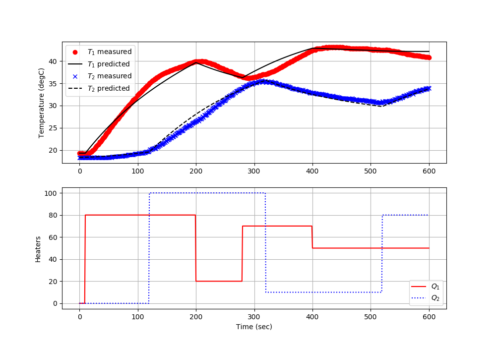
2nd Order System Identification
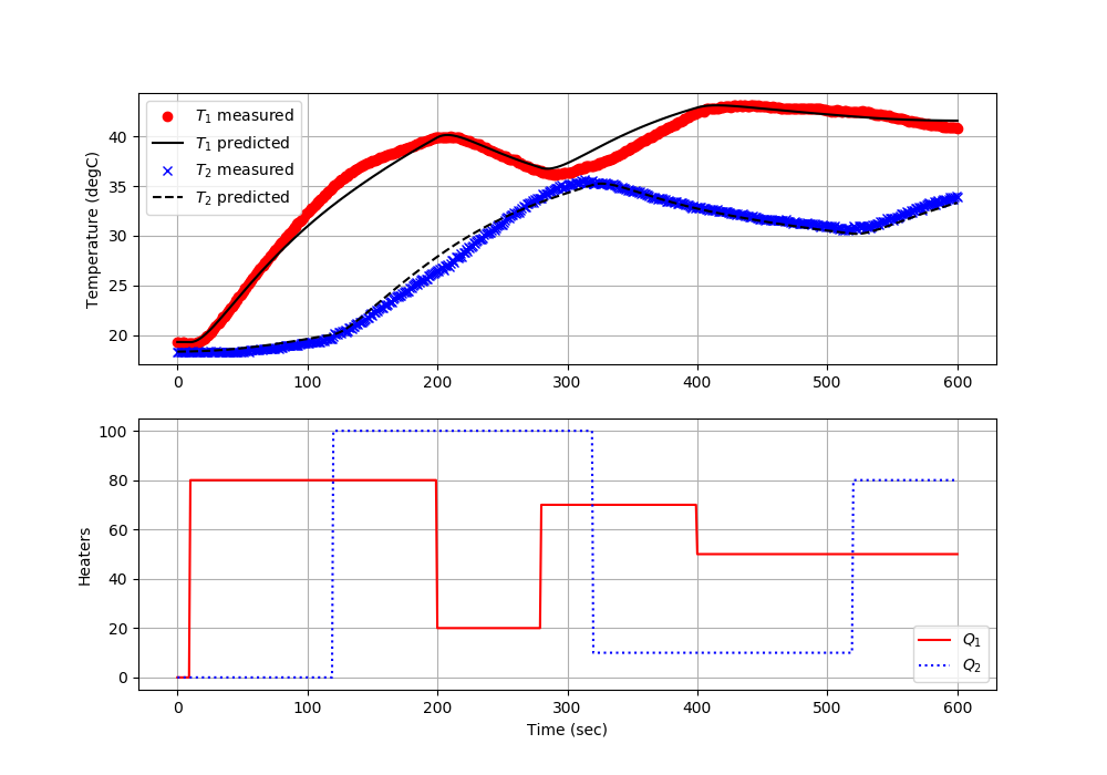
See information on .
(:toggle hide gekko_labD2 button show="Lab D: Python GEKKO 2nd Order":) (:div id=gekko_labD2:) import numpy as np import time import matplotlib.pyplot as plt import random
- get gekko package with:
- pip install gekko
from gekko import GEKKO import pandas as pd
- import data
try:
    # read data file if available
    data = pd.read_csv('tclab_dyn_data2.csv')
except:
    # retrieve data file from Internet source
    url = 'http://apmonitor.com/do/uploads/Main/tclab_dyn_data2.txt'
    data = pd.read_csv(url)
tm = data['Time'].values Q1s = data['H1'].values # heater 1 Q2s = data['H2'].values # heater 2 T1s = data['T1'].values T2s = data['T2'].values
- Initialize Model as Estimator
m = GEKKO(remote=True)
m.time = tm
- Parameters to Estimate
K1 = m.FV(value=0.5,lb=0.1,ub=1.0) K2 = m.FV(value=0.3,lb=0.1,ub=1.0) K3 = m.FV(value=0.1,lb=0.0001,ub=1.0) tau12 = m.FV(value=150,lb=50,ub=250) tau3 = m.FV(value=15,lb=10,ub=20)
K1.STATUS = 1 K2.STATUS = 1 K3.STATUS = 1 tau12.STATUS = 1 tau3.STATUS = 1
- Measured inputs
Q1 = m.MV(value=Q1s) Q2 = m.MV(value=Q2s)
- use measurements
Q1.FSTATUS = 1 # measured Q2.FSTATUS = 1 # measured
- Ambient temperature
Ta = m.Param(value=19.0) # degC
- State variables
TH1 = m.SV(value=T1s[0]) TH2 = m.SV(value=T2s[0])
- Measurements for model alignment
TC1 = m.CV(value=T1s) TC1.STATUS = 1 # minimize error between simulation and measurement TC1.FSTATUS = 1 # receive measurement TC1.MEAS_GAP = 0.1 # measurement deadband gap
TC2 = m.CV(value=T2s) TC2.STATUS = 1 # minimize error between simulation and measurement TC2.FSTATUS = 1 # receive measurement TC2.MEAS_GAP = 0.1 # measurement deadband gap
- Heat transfer between two heaters
DT = m.Intermediate(TH2-TH1)
- Empirical correlations
m.Equation(tau12 * TH1.dt() + (TH1-Ta) == K1*Q1 + K3*DT) m.Equation(tau12 * TH2.dt() + (TH2-Ta) == K2*Q2 - K3*DT) m.Equation(tau3 * TC1.dt() + TC1 == TH1) m.Equation(tau3 * TC2.dt() + TC2 == TH2)
- Global Options
m.options.IMODE = 5 # MHE m.options.EV_TYPE = 2 # Objective type m.options.NODES = 3 # Collocation nodes m.options.SOLVER = 3 # IPOPT
- Predict Parameters and Temperatures
m.solve()
- Create plot
plt.figure(figsize=(10,7))
ax=plt.subplot(2,1,1) ax.grid() plt.plot(tm,T1s,'ro',label=r'$T_1$ measured') plt.plot(tm,TC1.value,'k-',label=r'$T_1$ predicted') plt.plot(tm,T2s,'bx',label=r'$T_2$ measured') plt.plot(tm,TC2.value,'k--',label=r'$T_2$ predicted') plt.ylabel('Temperature (degC)') plt.legend(loc=2) ax=plt.subplot(2,1,2) ax.grid() plt.plot(tm,Q1s,'r-',label=r'$Q_1$') plt.plot(tm,Q2s,'b:',label=r'$Q_2$') plt.ylabel('Heaters') plt.xlabel('Time (sec)') plt.legend(loc='best')
- Print optimal values
print('K1: ' + str(K1.newval)) print('K2: ' + str(K2.newval)) print('K3: ' + str(K3.newval)) print('tau12: ' + str(tau12.newval)) print('tau3: ' + str(tau3.newval))
- Save and show figure
plt.savefig('tclab_2nd_order.png') plt.show() (:source lang=python:) (:sourceend:) (:divend:)
See also:
Advanced Control Lab Overview
GEKKO Documentation
TCLab Documentation
TCLab Files on GitHub
Basic (PID) Control Lab
(:html:) <style> .button {
  border-radius: 4px;
  background-color: #0000ff;
  border: none;
  color: #FFFFFF;
  text-align: center;
  font-size: 28px;
  padding: 20px;
  width: 300px;
  transition: all 0.5s;
  cursor: pointer;
  margin: 5px;
}
.button span {
  cursor: pointer;
  display: inline-block;
  position: relative;
  transition: 0.5s;
}
.button span:after {
  content: '\00bb';
  position: absolute;
  opacity: 0;
  top: 0;
  right: -20px;
  transition: 0.5s;
}
.button:hover span {
padding-right: 25px;
}
.button:hover span:after {
  opacity: 1;
  right: 0;
} </style> (:htmlend:)