Dynamic Optimization

Temperature control is crucial for maximizing ethanol production, as it directly affects yeast activity and fermentation efficiency. Most ethanol-producing yeasts thrive within an optimal temperature range, typically 30–35°C, where metabolic activity and ethanol yield are maximized. Deviation from this range can slow fermentation or cause thermal stress, reducing cell viability and ethanol production. Bioreactors often use temperature-regulating systems, such as water jackets, heat exchangers, or cooling coils, to maintain the ideal temperature. In large-scale operations, active cooling is essential to counteract heat generated during fermentation. Precise temperature control also helps minimize the production of unwanted by-products and supports consistent ethanol yields. Automated systems with temperature sensors and feedback controls are frequently employed to ensure stable conditions throughout the process.

Ethanol bioreactors can strategically use air to optimize production by supporting yeast health and process efficiency. During initial stages, oxygen is introduced to promote yeast propagation, enhancing cell growth and the production of sterols and fatty acids essential for robust fermentation. Some systems maintain microaerophilic conditions, carefully controlling oxygen levels to balance yeast growth and ethanol synthesis, as excessive oxygen shifts metabolism toward biomass production rather than ethanol. In certain setups, aerobic bacteria are co-cultured with yeast to degrade inhibitors like furfural or acetic acid, improving overall efficiency. Aeration is also used to manage heat and CO₂ accumulation in large-scale systems, though excessive oxygen must be avoided to preserve yields. While fermentation is primarily anaerobic, these controlled applications of air can enhance production by optimizing the fermentation environment.

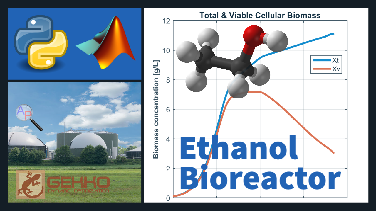
(:html:) <iframe width="560" height="315" src="https://www.youtube.com/embed/n2o1Cx5_pwo" frameborder="0" allow="accelerometer; autoplay; clipboard-write; encrypted-media; gyroscope; picture-in-picture" allowfullscreen></iframe> (:htmlend:)

• Bioreactor Simulation for Ethanol Production using GEKKO, Stack Overflow, Nov 9, 2022.

1. Specify values of control variables [Qin0 Qin Xtin Xvin Qe Sin Fc Fair Tin Tcin]

(:sourceend:) (:divend:)

Optimize Ethanol Production

The simulation model of an ethanol bioreactor can be used to optimize the production of ethanol by providing a virtual platform to test different scenarios and strategies without the need for costly and time-consuming experimental trials. Follow these steps to optimize the ethanol production:

1. Define the parameters: Once the model is built, the next step is to define the parameters that affect the production of ethanol. These may include variables such as temperature, substrate concentration, batch time, and other relevant variables.
2. Run simulations: Using the defined parameters, run simulations to determine the best conditions for maximizing ethanol production. The simulations can be run repeatedly, each time changing one or more variables to determine the optimal combination.
3. Analyze the results: After running the simulations, analyze the results to identify the optimal conditions for maximizing ethanol production. The analysis can be done using statistical techniques or data visualization tools to help identify trends and patterns.
4. Optimize the bioreactor: Based on the results of the analysis, optimize the bioreactor operation by adjusting the parameters to the identified optimal conditions. This may involve adjusting the reactor temperature, substrate concentration, or other variables.
5. Validate the model: test the simulation model by comparing the results obtained from the simulation with experimental data obtained from the actual bioreactor. This ensures that the results of the optimization are accurate.

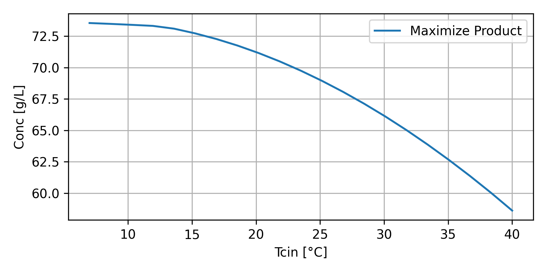
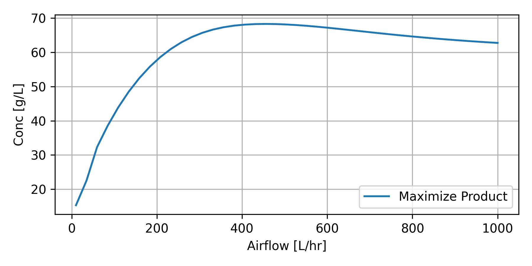
The optimization strategy is used to determine the optimal Tcin (temperature to the cooling jacket) and Fair (air flow).

Maximize Ethanol Production with Cooling Temperature

bioreactor_Tcin.png

Maximize Ethanol Production with Air Flow Rate

bioreactor_Fair.png

(:toggle hide opt_odeint button show="Show Python ODEINT Code":) (:div id=opt_odeint:) (:source lang=python:) import numpy as np from scipy.integrate import odeint from scipy.interpolate import interp1d import matplotlib.pyplot as plt

1. Simulate fed-batch operation
2. Specify the simulation time (hrs)

tspan = np.linspace(0,37,371); t=tspan

1. Specify values of control variables [Qin0 Qin Xtin Xvin Qe Sin Fc Fair Tin Tcin]

u0 = [0.0,0.0,0.0,0.0,0.0,400,40,60000,30,15]

1. Specify initial conditions [Xt Xv S P Oliq Ogas T Tc Vl Gloss MP]

x0 = [0.1,0.1,50,0,0.0065,0.305,30,20,1000,0.0,0.0] ux0 = (u0 + x0)

1. Qin = 15*heaviside(t-5) + 5*heaviside(t-10)
2. - 6*heaviside(t-20) - 14*heaviside(t-35)

Qin = np.zeros_like(tspan) Qin[np.where(tspan>=5)] += 15 Qin[np.where(tspan>=10)] += 5 Qin[np.where(tspan>=20)] -= 6 Qin[np.where(tspan>=35)] -= 14 QinInterp = interp1d(tspan,Qin,bounds_error=False)

def ethanol(x,t,Qin0,Qin,Xtin,Xvin,Qe,Sin,Fc,Fair,

            Tin,Tcin,Xt0,Xv0,S0,P0,Oliq0,Ogas0,T0,
            Tc0,Vl0,Sf_cum0,Time0):
    ##    #Initial Conditions
    ##    Xt0 = u[10]     # Initial total cellular biomass, [g L-1]
    ##    Xv0 = u[11]     # Initial viable cellular biomass, [g L-1]
    ##    S0 = u[12]      # Initial substrate/Glucose concentration, [g L-1]
    ##    P0 = u[13]      # Initial product/Ethanol concentration, [g L-1]
    ##    Oliq0 = u[14]   # Initial Dissolved oxygen concentration, [g L-1]
    ##    Ogas0 = u[15]   # Initial Gas phase oxygen (bubbles) in the fermentation broth, [g L-1]
    ##    T0 = u[16]      # Initial Temperature in the bioreactor, [oC]
    ##    Tc0 = u[17]     # Initial Temperature of the cooling agent in the jacket, [oC]
    ##    Vl0 = u[18]     # Initial Culture volume in the bioreactor, [L]
    ##    Sf_cum0 = u[19] # Initial Cumulative substrate/glucose fed to the bioreactor, [g]
    ##    Time0 = u[20]   # Initial batch time, [h]
    ##    
    ##    #Control variables
    ##    Qin0 = u[0]        # Volumetric inflow rate, [l/h-1]
    ##    Qin = u[1]         # Volumetric inflow rate, [l/h-1]
    ##    Xtin = u[2]        # Total biomass concentration in the bioreactor feed, [g L-1]
    ##    Xvin = u[3]        # Viable biomass concentration in the bioreactor feed, [g L-1]
    ##    Qe = u[4]          # Volumetric outflow rate, [l/h-1]
    ##    Sin = u[5]         # Substrate/Glucose concentration in bioreactor feed, [g L-1]
    ##    Fc = u[6]          # Cooling agent inlet volumetric flowrate, [L h-1]
    ##    Fair = u[7]        # Airflow inlet volumetric flowrate, [L h-1]
    ##    Tin = u[8]         # Temperature of bioreactor feed, [oC]
    ##    Tcin = u[9]        # Temperature of cooling agent inlet, [oC]

    # 1D Interpolation for Qin
    Qin = QinInterp(t)

    #Definition of model parameters
    #Kinetic parameters
    a1 = 0.05    # Ratkowsky parameter [oC-1 h-0.5]
    aP = 4.50    # Growth-associated parameter for ethanol production, [-]
    AP1 = 6.0    # Activation energy parameter for ethanol production, [oC]
    AP2 = 20.3   # Activation energy parameter for ethanol production, [oC]
    b1 = 0.035   # Parameter in the exponential expression of the maximum specific growth rate np.expression, [oC-1]
    b2 = 0.15    # Parameter in the exponential expression of the growth inhibitory ethanol concentration np.expression, [oC-1]
    b3 = 0.40    # Parameter in the exponential np.expression of the specific death rate expression,[oC-1]
    c1 = 0.38    # Constant decoupling factor for ethanol production, [gP gX-1 h-1]
    c2 = 0.29    # Constant decoupling factor for ethanol production, [gP gX-1 h-1]
    k1 = 3.00    # Parameter in the maximum specific growth rate expression, [oC]
    k2 = 55.0    # Parameter in the maximum specific growth rate expression, [oC]
    k3 = 60.0    # Parameter in the growth-inhibitory ethanol concentration expression, [oC]
    k4 = 50.0    # Temperature at the inflection point of the specific death rate sigmoid curve, [oC]
    Pmaxb = 90   # Temperature-independent product inhibition constant, [g L-1]
    PmaxT = 90   # Maximum value of product inhibition constant due to temperature, [g L-1]
    Kdb = 0.025  # Basal specific cellular biomass death rate, [h-1]
    KdT = 30.00  # Maximum value of specific cellular biomass death rate due to temperature, [h-1]
    KSX = 5      # Glucose saturation constant for the specific growth rate, [g L-1]
    KOX = 0.0005 # Oxygen saturation constant for the specific growth rate, [g L-1]
    qOmax = 0.05 # Maximum specific oxygen consumption rate, [h-1]

    #Metabolic parameters
    YPS = 0.51 # Theoretical yield of ethanol on glucose, [gP gS-1]
    YXO = 0.97 # Theoretical yield of biomass on oxygen, [gX gO-1]
    YXS = 0.53 # Theoretical yield of biomass on glucose, [gX gS-1]

    #Physicochemical and thermodynamic parameters
    Chbr = 4.18     # Heat capacity of the mass of reaction, [J g-1 oC-1]
    Chc = 4.18      # Heat capacity of the cooling agent, [J g-1 oC-1]
    DeltaH = 518000 # Heat of reaction of fermentation, [J mol-1 O2]
    Tref = 20       # Reference temperature, [oC]
    KH = 200        # Henry's constant for oxygen in the fermentation broth, [atm L mol-1]
    z = 0.792       # Oxygen compressibility factor, [-]
    R = 0.082       # Ideas gas constant, [L atm mol-1 oC-1]
    kla0 = 100      # Temperature-independent volumetric oxygen transfer coefficient, [h-1]
    KT = 360000     # Heat transfer coefficient, [J h-1 m-2 ??C-1]
    rho = 1080      # Density of the fermentation broth, [g L-1]
    rhoc = 1000     # Density of the cooling agent, [g L-1]
    MO = 32.0       # Molecular weight of oxygen (O2), [g mol-1]

    #Bioreactor design data
    AT = 1.0       # Bioreactor heat transfer area, [m2]
    V = 1800       # Bioreactor working volume, [L]
    Vcj = 50       # Cooling jacket volume, [L]
    Ogasin = 0.305 # Oxygen concentration in airflow inlet, [g L-1]

    #Definition of model variables
    #State variables
    Xt = x[0]      # Total cellular biomass, [g L-1]
    Xv = x[1]      # Viable cellular biomass, [g L-1]
    S = x[2]       # Substrate/Glucose concentration, [g L-1]
    P = x[3]       # Product/Ethanol concentration, [g L-1]
    Oliq = x[4]    # Dissolved oxygen concentration, [g L-1]
    Ogas = x[5]    # Gas phase oxygen (bubbles) in the fermentation broth, [g L-1]
    T = x[6]       # Temperature in the bioreactor, [oC]
    Tc = x[7]      # Temperature of the cooling agent in the jacket, [oC]
    Vl = x[8]      # Culture volume in the bioreactor, [L]
    Sf_cum = x[9]  # Cumulative amount of substrate/glucose fed to the bioreactor, [g]
    Time = x[10]   # Batch time, [h]

    # Definition of model equations
    # Kinetic rates
    # -----------------------------
    # Specific growth rate, [h-1] 
    mmax = ((a1*(T-k1))*(1-np.exp(b1*(T-k2))))**2
    Pmax = Pmaxb + PmaxT/(1-np.exp(-b2*(T-k3)))
    m1 = mmax * S/(KSX + S) * Oliq/(KOX + Oliq) * (1 - P/Pmax) * 1/(1+np.exp(-(100-S)/1)) # Specific growth rate, [h-1] 
    if m1 >= 0:
        m = m1
    else:
        m=0.0
    # Non-growth-associated ethanol specific production rate, [h-1]
    if S > 0:
        bP = c1 * np.exp(-AP1/T) - c2 * np.exp(-AP2/T)  # Non-growth-associated ethanol specific production rate, [h-1]
    else:
        bP = 0.0
    qP = aP*m + bP
    # Ethanol consumption specific rate
    qS = m/YXS + qP/YPS
    # Oxygen consumption specific rate
    qO = qOmax*Oliq/YXO/(KOX + Oliq)
    # Specific biological deactivation rate of cell mass
    Kd = Kdb + KdT/(1+np.exp(-b3*(T-k4)))
    # Saturation concentration of oxygen in culture media
    Osat = z*Ogas*R*T/KH
    # Oxygen mass transfer coefficient
    kla = kla0*1.2**(T-20)
    # Volume of the gas phase in the bioreactor
    Vg = V - Vl

    #Material balances
    #-----------------
    # Volume of liquid culture
    dVl = Qin - Qe
    # Total cell mass
    dXt = m*Xv + Qin/Vl*(Xtin-Xt)
    # Total mass of biologically active cells
    dXv = (m-Kd)*Xv + Qin/Vl*(Xvin-Xv)
    # Glucose concentration
    dS = Qin/Vl*(Sin-S) - qS*Xv
    # Ethanol concentration
    dP = Qin/Vl*(-P) + qP*Xv
    # Disolved oxygen
    dOliq = Qin/Vl*(Osat - Oliq) + kla*(Osat-Oliq) - qO*Xv
    # Oxygen gas phase
    dOgas = Fair/Vg*(Ogasin-Ogas) - Vl*kla/Vg*(Osat - Oliq) + Ogas*(Qin-Qe)/Vg

    # Energy balances
    #---------------
    # Bioreactor temprature
    dT = Qin/Vl*(Tin-T) - Tref/Vl*(Qin-Qe) + qO*Xv*DeltaH/MO/rho/Chbr - KT*AT*(T-Tc)/Vl/rho/Chbr
    # Cooling agent temperature
    dTc = Fc/Vcj*(Tcin-Tc) + KT*AT*(T-Tc)/Vcj/rhoc/Chc

    # Yields & Productivity
    #---------------------
    # Cumulative amount of glucose fed to the bioreactor
    dSf_cum = Sin*Qin
    dTime = 1

    # Definition of state derivatives vector
    # State derivatives
    dxdt = [dXt,dXv,dS,dP,dOliq,dOgas,dT,dTc,dVl,dSf_cum,dTime]

    return dxdt

T_val = np.linspace(7,40,21) P_val = np.empty_like(T_val) ux1 = ux0 for i,T in enumerate(T_val):

    ux1[9] = T
    x = odeint(ethanol,x0,tspan,args=tuple(ux1))
    P_val[i] = x[-3,3]

plt.figure(figsize=(6,3)) plt.plot(T_val, P_val, label='Maximize Product') plt.legend(); plt.grid() plt.ylabel('Conc [g/L]') plt.xlabel('Tcin') plt.tight_layout() plt.savefig('bioreactor_Tcin.png',dpi=300)

F_val = np.linspace(10,1000,41) P_val = np.empty_like(F_val) ux2 = ux0 for i,F in enumerate(F_val):

    ux2[7] = F
    x = odeint(ethanol,x0,tspan,args=tuple(ux2))
    P_val[i] = x[-3,3]

plt.figure(figsize=(6,3)) plt.plot(F_val, P_val, label='Maximize Product') plt.legend(); plt.grid() plt.ylabel('Conc [g/L]') plt.xlabel('Airflow [L/hr]') plt.tight_layout() plt.savefig('bioreactor_Fair.png',dpi=300) plt.show()

a1 = 0.05 # Ratkowsky parameter [oC-1 h-0.5] aP = 4.50 # Growth-associated parameter for EtOh production [-] AP1 = 6.0 # Activation energy parameter for EtOh production [oC] AP2 = 20.3 # Activation energy parameter for EtOh production [oC] b1 = 0.035 # Parameter in the exponential expression of the maximum specific growth rate expression [oC-1] b2 = 0.15 # Parameter in the exponential expression of the maximum specific growth rate expression [oC-1] b3 = 0.40 # Parameter in the exponential expression of the specific death rate expression [oC-1] c1 = 0.38 # Constant decoupling factor for EtOh [gP gX-1 h-1] c2 = 0.29 # Constant decoupling factor for EtOh [gP gX-1 h-1] k1 = 3 # Parameter in the maximum specific growth rate expression [oC] k2 = 55 # Parameter in the maximum specific growth rate expression [oC] k3 = 60 # Parameter in the growth-inhibitory EtOH concentration expression [oC] k4 = 50 # Temperature at the inflection point of the specific death rate sigmoid curve [oC] Pmaxb = 90 # Temperature-independent product inhibition constant [g L-1] PmaxT = 90 # Maximum value of product inhibition constant due to temperature [g L-1] Kdb = 0.025 # Basal specific cellular biomass death rate [h-1] KdT = 30 # Maximum value of specific cellular biomass death rate due to temperature [h-1] KSX = 5 # Glucose saturation constant for the specific growth rate [g L-1] KOX = 0.0005 # Oxygen saturation constant for the specific growth rate [g L-1] qOmax = 0.05 # Maximum specific oxygen consumption rate [h-1]

YPS = 0.51 # Theoretical yield of EtOH on glucose [gP gS-1] YXO = 0.97 # Theoretical yield of biomass on oxygen [gX gO-1] YXS = 0.53 # Theoretical yield of biomass on glucose [gX gS-1]

Chbr = 4.18 # Heat capacity of the mass of reaction [J g-1 oC-1] Chc = 4.18 # Heat capacity of cooling agent [J g-1 oC-1] deltaH = 518000 # Heat of reaction of fermentation [J mol-1 O2] Tref = 20 # Reference temperature [oC] KH = 200 # Henry's constant for oxygen in the fermentation broth [atm L mol-1] z = 0.792 # Oxygen compressibility factor [-] R = 0.082 # Ideal gas constant [L atm mol-1 oC-1] kla0 = 100 # Temperature-independent volumetric oxygen transfer coefficient [-h] KT = 360000 # Heat transfer coefficient [J h-1 m-2 oC-1] rho = 1080 # Density of the fermentation broth [g L-1] rhoc = 1000 # Density of the cooling agent [g L-1] MO = 32.0 # Molecular weight of oxygen [g mol-1]

AT = 1 # Bioreactor heat transfer area [m2] V = 1800 # Bioreactor working volume [L] Vcj = 50 # Cooling jacket volume [L] Ogasin = 0.305 # Oxygen concentration in airflow inlet [g L-1]

1. Qin is a step function:

plt.plot(m.time, P.value, label='P')

One particular batch bioreactor is fed at varying rates throughout the batch process to produce ethanol. Algebraic equations define the heat generation, rate constants, volume, and other factors used in the model. Symbols and units are defined in the source code.

Growth Rate

Non-Growth Ethanol Production

Ethanol Consumption Rate

Oxygen Consumption Rate

Biological Cell Mass Deactivation Rate

Oxygen Saturation Concentration

Oxygen Mass Transfer Coefficient

$${k}_{l} {a}=\left({k}_{l} {a}\right)_0(1.2)^{{T}-20}$$

Liquid and Vapor Volumes

Differential equations are from material, species, and energy balances. The differential equations relate the input flow and substrate concentrations to ethanol production.

Liquid Volume

Total Cell Mass

Total Biologically Active Cell Mass

Glucose (Substrate) Concentration

Ethanol (Product) Concentration

Liquid Oxygen Concentration

$$\frac{{dO}_{liq}}{{dt}}=\frac{{Q}_{{in}}}{{V}_{{l}}}\left({O}^*-{O}_{{liq}}\right)+\left({k}_{{l}} {a}\right)\left({O}^*-{O}_{{liq}}\right)-{qo}_{{o}} {X}_{{v}}$$

Gas Oxygen Concentration

Bioreactor Temperature

Cooling Agent Temperature

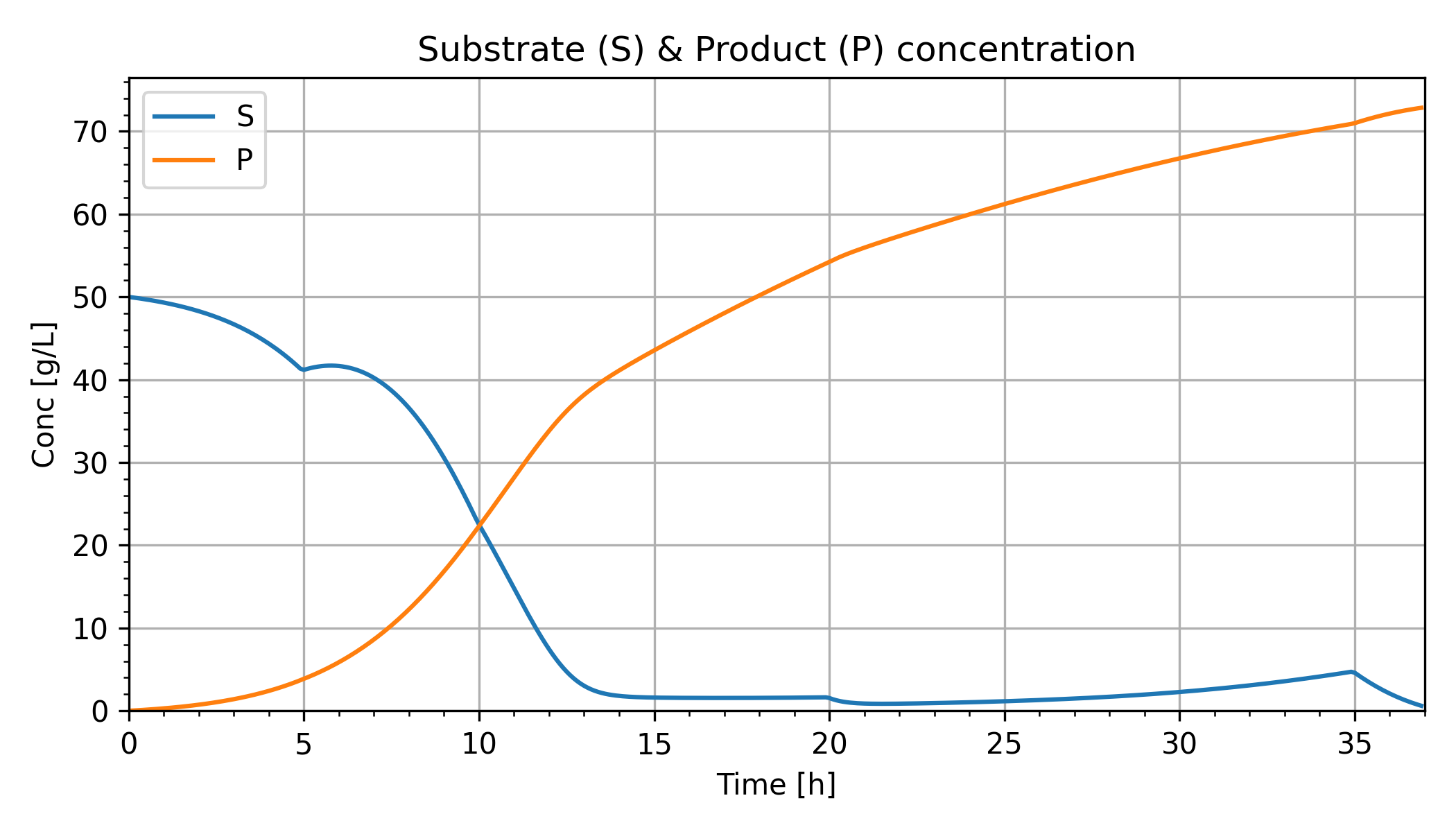
The model simulates biomass, ethanol, and by-product production. The following chart show total biomass and viable (living) biomass in the reactor.

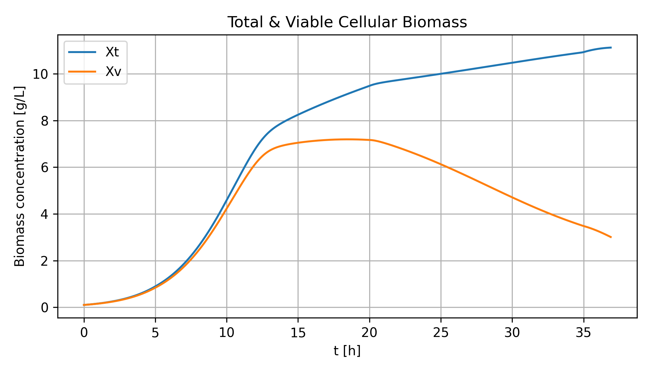
The model can be used to investigate advanced process control to maximize performance subject to a feeding strategy and measured disturbances.

plt.figure(figsize=(7,4))

plt.grid()

plt.tight_layout()

plt.figure(figsize=(7,4))

Save as reactor.m

clear; clc; close all; %Simulate fed-batch operation for xx hours % Specify the simulation time tspan = [0 37]; % Specify values of control variables [Qin0; Xtin; Xvin; Qe; Sin; Fc; Fair; Tin; Tcin] u0 = [0.0; 0.0; 0.0; 0.0; 400; 40; 60000; 30; 15]; % Specify initial conditions [Xt; Xv; S; P; Oliq; Ogas; T; Tc; Vl; Gloss; MP] x0 = [0.1; 0.1; 50; 0; 0.0065; 0.305; 30; 20; 1000; 0.0; 0.0]; ux0 = [u0;x0]; % Simulate the bioreactor operation until the selected time tf [t,x] = ode15s(@EthanolModel,tspan,x0,[],ux0); N=length(t); for i=1:size(t,1) [~,mmax(i,:),Pmax(i,:),bP(i,:),m(i,:),Kd(i,:),Qin(i,:)] = EthanolModel(t(i,:),x(i,:),ux0); end % Loss of substrate at the end of the bioreactor operation-Cumulative ethanol mass produced Gloss = x(N,3)*x(N,9);

%plots Results %Total and Viable Cellular Biomass figure(1) f=plot(t,x(:,1), t,x(:,2)); set(gca,'linewidth',1,'fontsize',12) set(f,'linewidth',3) grid title('Total & Viable Cellular Biomass') ylabel('Biomass concentration [g/L]','FontSize',12,'FontWeight', 'bold') xlabel('t [h]','FontSize', 12, 'FontWeight','bold') legend('Xt','Xv')

%Substrate(S) and Production(P) concentration figure(2) f=plot(t,x(:,3),'y', t,x(:,4),'g'); set(gca,'linewidth',1,'fontsize',12) set(f,'linewidth',3) grid title('Substrate (S) & Product (P) concetration') ylabel('Concentration [g/L]','FontSize',12,'FontWeight', 'bold') xlabel('t [h]','FontSize', 12, 'FontWeight','bold') legend('S','P')

% Dissolved and gaseous oxygen concentration figure(3) title('Dissolved and Gaseous oxygen concentration') hold on yyaxis left f=plot(t,x(:,5),'color',[0.3010 0.7450 0.9330]); set(gca,'linewidth',1,'fontsize',12) set(f,'linewidth',3) grid on ylabel('Oliq [g/L]','FontSize',12,'FontWeight', 'bold', 'color',[0.3010 0.7450 0.9330]) yyaxis right f=plot(t,x(:,6),'color',[250/255 128/255 114/255]); set(gca,'linewidth',1,'fontsize',12) set(f,'linewidth',3) grid on ylabel('Ogas [g/L]','FontSize',12,'FontWeight', 'bold','color',[250/255 128/255 114/255]) xlabel('t [h]','FontSize', 12, 'FontWeight','bold') legend('Oliq','Ogas') hold off

% Bioreactor & Cooling jacket temperature figure(4) f=plot(t,x(:,7), t,x(:,8)); set(gca,'linewidth',1,'fontsize',12) set(f,'linewidth',3) grid title('Bioreactor & Cooling jacket temperature') ylabel('Temperature [oC]','FontSize',12,'FontWeight', 'bold') xlabel('t [h]','FontSize', 12, 'FontWeight','bold') legend('T','Tc')

% Specific growth and death rate figure(5) f=plot(t,mmax, t,m, t,Kd); set(gca,'linewidth',1,'fontsize',12) set(f,'linewidth',3) grid title('Specific growth and death rate') ylabel('Specific growth and death rate [1/h]','FontSize',12,'FontWeight', 'bold') xlabel('t [h]','FontSize', 12, 'FontWeight','bold') legend('mimax','mi','Kd')

% Production rate figure(6) title('Production rate') hold on yyaxis left f=plot(t,bP); set(gca,'linewidth',1,'fontsize',12) set(f,'linewidth',3) grid on ylabel('bP [1/h]','FontSize',12,'FontWeight', 'bold') yyaxis right f=plot(t,Pmax); set(gca,'linewidth',1,'fontsize',12) set(f,'linewidth',3) grid on ylabel('Pmax','FontSize',12,'FontWeight', 'bold') xlabel('t [h]','FontSize', 12, 'FontWeight','bold') legend('bP','Pmax') hold off

% Culture Volume & Total substrate fed to the BR figure(7) title('Culture Volume & Total substrate fed to the BR') hold on yyaxis left f=plot(t,x(:,9)); set(gca,'linewidth',1,'fontsize',12) set(f,'linewidth',3) grid on ylabel('Vl [L]','FontSize',12,'FontWeight', 'bold') yyaxis right f=plot(t,x(:,10)); set(gca,'linewidth',1,'fontsize',12) set(f,'linewidth',3) grid on ylabel('Sf_cum [g]','FontSize',12,'FontWeight', 'bold') xlabel('t [h]','FontSize', 12, 'FontWeight','bold') legend('Vl','Sf_cum') hold off

% Feeding Policy figure(8) title('Feeding policy') f=plot(t,Qin); set(gca,'linewidth',1,'fontsize',12) set(f,'linewidth',3) grid on ylabel('Qin [L/h]','FontSize',12,'FontWeight', 'bold') xlabel('t [h]','FontSize', 12, 'FontWeight','bold') legend('Qin')

Save as EthanolModel.m

function [dxdt,mmax,Pmax,bP,m,Kd,Qin] = EthanolModel(t,x,u) %Definition of model parameters %Kinetic parameters a1 = 0.05; % Ratkowsky parameter [oC-1 h-0.5] aP = 4.50; % Growth-associated parameter for ethanol production, [-] AP1 = 6.0; % Activation energy parameter for ethanol production, [oC] AP2 = 20.3; % Activation energy parameter for ethanol production, [oC] b1 = 0.035; % Parameter in the exponential expression of the maximum specific growth rate expression, [oC-1] b2 = 0.15; % Parameter in the exponential expression of the growth inhibitory ethanol concentration expression, [oC-1] b3 = 0.40; % Parameter in the exponential expression of the specific death rate expression,[oC-1] c1 = 0.38; % Constant decoupling factor for ethanol production, [gP gX-1 h-1] c2 = 0.29; % Constant decoupling factor for ethanol production, [gP gX-1 h-1] k1 = 3.00; % Parameter in the maximum specific growth rate expression, [oC] k2 = 55.0; % Parameter in the maximum specific growth rate expression, [oC] k3 = 60.0; % Parameter in the growth-inhibitory ethanol concentration expression, [oC] k4 = 50.0; % Temperature at the inflection point of the specific death rate sigmoid curve, [oC] Pmaxb = 90; % Temperature-independent product inhibition constant, [g L-1] PmaxT = 90; % Maximum value of product inhibition constant due to temperature, [g L-1] Kdb = 0.025; % Basal specific cellular biomass death rate, [h-1] KdT = 30.00; % Maximum value of specific cellular biomass death rate due to temperature, [h-1] KSX = 5; % Glucose saturation constant for the specific growth rate, [g L-1] KOX = 0.0005; % Oxygen saturation constant for the specific growth rate, [g L-1] qOmax = 0.05; % Maximum specific oxygen consumption rate, [h-1]

%Metabolic parameters YPS = 0.51; % Theoretical yield of ethanol on glucose, [gP gS-1] YXO = 0.97; % Theoretical yield of biomass on oxygen, [gX gO-1] YXS = 0.53; % Theoretical yield of biomass on glucose, [gX gS-1]

%Physicochemical and thermodynamic parameters Chbr = 4.18; % Heat capacity of the mass of reaction, [J g-1 oC-1] Chc = 4.18; % Heat capacity of the cooling agent, [J g-1 oC-1] DeltaH = 518000; % Heat of reaction of fermentation, [J mol-1 O2] Tref = 20; % Reference temperature, [oC] KH = 200; % Henry's constant for oxygen in the fermentation broth, [atm L mol-1] z = 0.792; % Oxygen compressibility factor, [-] R = 0.082; % Ideas gas constant, [L atm mol-1 oC-1] kla0 = 100 ; % Temperature-independent volumetric oxygen transfer coefficient, [h-1] KT = 360000; % Heat transfer coefficient, [J h-1 m-2 ??C-1] rho = 1080 ; % Density of the fermentation broth, [g L-1] rhoc = 1000 ; % Density of the cooling agent, [g L-1] MO = 32.0; % Molecular weight of oxygen (O2), [g mol-1]

%Bioreactor design data AT = 1.0; % Bioreactor heat transfer area, [m2] V = 1800; % Bioreactor working volume, [L] Vcj = 50; % Cooling jacket volume, [L] Ogasin = 0.305; % Oxygen concentration in airflow inlet, [g L-1]

%Definition of model variables %State variables Xt = x(1); % Total cellular biomass, [g L-1] Xv = x(2); % Viable cellular biomass, [g L-1] S = x(3); % Substrate/Glucose concentration, [g L-1] P = x(4); % Product/Ethanol concentration, [g L-1] Oliq = x(5); % Dissolved oxygen concentration, [g L-1] Ogas = x(6); % Gas phase oxygen (bubbles) in the fermentation broth, [g L-1] T = x(7); % Temperature in the bioreactor, [oC] Tc = x(8); % Temperature of the cooling agent in the jacket, [oC] Vl = x(9); % Culture volume in the bioreactor, [L] Sf_cum = x(10); % Cumulative amount of substrate/glucose fed to the bioreactor, [g] Time = x(11); % Batch time, [h]

%Initial Conditions Xt0 = u(10); % Initial total cellular biomass, [g L-1] Xv0 = u(11); % Initial viable cellular biomass, [g L-1] S0 = u(12); % Initial substrate/Glucose concentration, [g L-1] P0 = u(13); % Initial product/Ethanol concentration, [g L-1] Oliq0 = u(14); % Initial Dissolved oxygen concentration, [g L-1] Ogas0 = u(15); % Initial Gas phase oxygen (bubbles) in the fermentation broth, [g L-1] T0 = u(16); % Initial Temperature in the bioreactor, [oC] Tc0 = u(17); % Initial Temperature of the cooling agent in the jacket, [oC] Vl0 = u(18); % Initial Culture volume in the bioreactor, [L] Sf_cum0 = u(19); % Initial Cumulative substrate/glucose fed to the bioreactor, [g] Time0 = u(20); % Initial batch time, [h]

%Control variables Qin0 = u(1); % Volumetric inflow rate, [l/h-1] Qin= Qin0 + 15*heaviside(t-5) + 5*heaviside(t-10) - 6*heaviside(t-20) - 14*heaviside(t-35); Xtin = u(2); % Total biomass concentration in the bioreactor feed, [g L-1] Xvin = u(3); % Viable biomass concentration in the bioreactor feed, [g L-1] Qe = u(4); % Volumetric outflow rate, [l/h-1] Sin = u(5); % Substrate/Glucose concentration in bioreactor feed, [g L-1] Fc = u(6); % Cooling agent inlet volumetric flowrate, [L h-1] Fair = u(7); % Airflow inlet volumetric flowrate, [L h-1] Tin = u(8); % Temperature of bioreactor feed, [oC] Tcin = u(9); % Temperature of cooling agent inlet, [oC]

% Definition of model equations % Kinetic rates % ----------------------------- % Specific growth rate, [h-1] mmax = ((a1*(T-k1))*(1-exp(b1*(T-k2))))^2; Pmax = Pmaxb + PmaxT/(1-exp(-b2*(T-k3))); m1 = mmax * S/(KSX + S) * Oliq/(KOX + Oliq) * (1 - P/Pmax) * 1/(1+exp(-(100-S)/1)); % Specific growth rate, [h-1] if m1 >= 0 m = m1; else m=0.0; end % Non-growth-associated ethanol specific production rate, [h-1] if S > 0 bP = c1 * exp(-AP1/T) - c2 * exp(-AP2/T) ; % Non-growth-associated ethanol specific production rate, [h-1] else bP = 0.0; end qP = aP*m + bP; % Ethanol consumption specific rate qS = m/YXS + qP/YPS; % Oxygen consumption specific rate qO = qOmax*Oliq/YXO/(KOX + Oliq); % Specific biological deactivation rate of cell mass Kd = Kdb + KdT/(1+exp(-b3*(T-k4))); % Saturation concentration of oxygen in culture media Osat = z*Ogas*R*T/KH; % Oxygen mass transfer coefficient kla = kla0*1.2^(T-20); % Volume of the gas phase in the bioreactor Vg = V - Vl;

%Material balances %----------------- % Volume of liquid culture dVl = Qin - Qe; % Total cell mass dXt = m*Xv + Qin/Vl*(Xtin-Xt); % Total mass of biologically active cells dXv = (m-Kd)*Xv + Qin/Vl*(Xvin-Xv); % Glucose concentration dS = Qin/Vl*(Sin-S) - qS*Xv; % Ethanol concentration dP = Qin/Vl*(-P) + qP*Xv; % Disolved oxygen dOliq = Qin/Vl*(Osat - Oliq) + kla*(Osat-Oliq) - qO*Xv; % Oxygen gas phase dOgas = Fair/Vg*(Ogasin-Ogas) - Vl*kla/Vg*(Osat - Oliq) + Ogas*(Qin-Qe)/Vg;

% Energy balances %--------------- % Bioreactor temprature dT = Qin/Vl*(Tin-T) - Tref/Vl*(Qin-Qe) + qO*Xv*DeltaH/MO/rho/Chbr - KT*AT*(T-Tc)/Vl/rho/Chbr; % Cooling agent temperature dTc = Fc/Vcj*(Tcin-Tc) + KT*AT*(T-Tc)/Vcj/rhoc/Chc;

% Yields & Productivity %--------------------- % Cumulative amount of glucose fed to the bioreactor dSf_cum = Sin*Qin; dTime = 1;

% Definition of state derivatives vector % State derivatives dxdt = [dXt; dXv; dS; dP; dOliq; dOgas; dT; dTc; dVl; dSf_cum; dTime]; return

• Bioreactor Simulation for Ethanol Production using GEKKO, Stack Overflow, Nov 9, 2022.

(:title Ethanol Bioreactor:)

(:description Bioreactor simulation and optimization of ethanol production:)

Bioreactors create a biologically active environment for the production of chemicals. A bioreactor is a vessel where organisms are grown and preferential products are produced by controlling the feed and temperature. Bioreactors can either be aerobic or anaerobic.

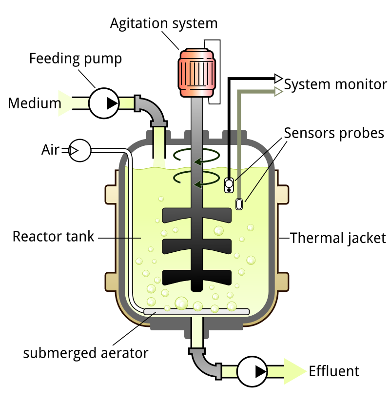
One particular batch bioreactor is fed at varying rates throughout the batch process to produce ethanol. Algebraic equations define the heat generation, kinetic rate constants, volume, and other factors used in the model. Symbols and units are defined in the source code.

$$\frac{d O_{{gas}}}{d t}=\frac{F_{{air}}}{V_g}\left(O_{{gas}, { in}}-O_{{gas}}\right)-\frac{V_l\left(k_l a\right)}{V_g}\left(O^*-O_{{liq}}\right)+O_{{gas}} \frac{Q_{{in}}-Q_e}{V_g}$$

(:title Fuel Ethanol Bioreactor:) (:keywords nonlinear, model, predictive control, APMonitor, gekko, differential, algebraic, modeling language, fuel ethanol, Process System Engineering:) (:description Bioreactor simulation and optimization of ethanol production:)

A batch bioreactor is fed at varying rates throughout the batch process to produce ethanol. Algebraic equations define the heat generation, kinetic rate constants, volume, and other factors used in the model. Symbols and units are defined in the source code.

$$\mu=\mu_{\max} \frac{{S}}{{K}_{{SX}}+{S}} \frac{{O}_{{liq}}}{{K}_{{OX}}+{O}_{{liq}}}\left(1-\frac{{P}}{{P}_{\max}}\right) \frac{1}{1+\exp (-(100-{S}))}$$

$$\mu_{\max}=\left[\left({a}_1\left({~T}-{k}_1\right)\right)\left(1-\exp \left({b}_1\left({~T}-{k}_2\right)\right)\right)\right]^2$$

$${P}_{\max}={P}_{\operatorname{maxb}}+\frac{{P}_{\operatorname{maxT}}}{1-\exp \left(-{b}_2\left({~T}-{k}_3\right)\right)}$$

$${q}_{{P}}={a}_{{P}} \mu+{b}_{{P}}$$

$${b}_{{P}}={c}_1 \exp \left(-\frac{{A}_{{P} 1}}{{~T}}\right)-{c}_2 \exp \left(-\frac{{A}_{{P} 2}}{{~T}}\right)$$

$${q}_{{S}}=\frac{\mu}{{Y}_{{XS}}}+\frac{{q}_{{P}}}{{Y}_{{PS}}}$$

$${q}_{{O}}=\frac{{q}_{{O}, \max}}{{Y}_{{Xo}}} \frac{{O}_{{liq}}}{{K}_{{OX}}+{O}_{{liq}}}$$

$${K}_{{d}}={K}_{{db}}+\frac{{K}_{{dT}}}{1+\exp \left(-{b}_3\left({~T}-{k}_4\right)\right)}$$

$${O}^*=\frac{{zO}_{{gas}} {RT}}{{K}_{{H}}}$$

$$\left({k}_{{l}} {a}\right)=\left({K}_{{l}} {a}\right)_0(1.2)^{{T}-20}$$

$${V}_{{l}}+{V}_{{g}}={V}$$

Differential equations are from material, species, and energy balances.

$$\frac{d V_1}{d t}=Q_{i n}-Q_e$$

$$\frac{{dX}}{{dt}}=\frac{{Q}_{{in}}}{{V}_1}\left({X}_{{t}, {in}}-{X}_{{t}}\right)+\mu {X}_{{v}}$$

$$\frac{d X_v}{d t}=\frac{Q_{i n}}{V_1}\left(X_{v, i n}-X_v\right)+\left(\mu-K_d\right) X_v$$

$$\frac{{dS}}{{dt}}=\frac{{Q}_{{in}}}{{V}_{{l}}}\left({S}_{{in}}-{S}\right)-{q}_{{S}} {X}_{{v}}$$

$$\frac{{dP}}{{dt}}=\frac{{Q}_{{in}}}{{V}_1}\left({P}_{{in}}-{P}\right)+{q}_{{P}} X_{{v}}$$

$$\frac{{dO} {liq}}{{dt}}=\frac{{Q}_{{in}}}{{V}_{{l}}}\left({O}^*-{O}_{{liq}}\right)+\left({k}_{{l}} {a}\right)\left({O}^*-{O}_{{liq}}\right)-{qo}_{{o}} {X}_{{v}}$$

$$\frac{d O_{{gas}}}{d t}=\frac{F_{{air}}}{V_g}\left(O_{{gas}, { in}}-O_{{gas}}\right)-\frac{V_l\left(k_l a\right)}{V_g}\left(0^*-O_{{liq}}\right)+O_{{gas}} \frac{Q_{{in}}-Q_e}{V_g}$$

$$\frac{{dT}}{{dt}}=\frac{{Q}_{{in}}}{{V}_{{l}}}\left({T}_{{in}}-{T}\right)-\frac{{T}_{{ref}}}{{V}_{{l}}}\left({Q}_{{in}}-{Q}_{{e}}\right)+\frac{{q}_{{o}} {X}_{{v}} \Delta {H}}{{MW}_{{O}} \rho {C}_{{p}, {br}}}-\frac{{K}_{{T}} {A}_{{T}}\left({T}-{T}_{{c}}\right)}{{V}_{{l}} \rho {C}_{{p}, {br}}}$$

$$\frac{{dT}_{{c}}}{{dt}}=\frac{{F}_{{c}}}{{V}_{{cj}}}\left({T}_{{c}, {in}}-{T}_{{c}}\right)+\frac{{K}_{{T}} {A}_{{T}}\left({T}-{T}_{{c}}\right)}{{V}_{{cj}} \rho_{{c}} {C}_{{p}, {c}}}$$

The model simulates biomass, ethanol, and by-product production. The model can be used to investigate advanced process control to maximize performance subject to a feeding strategy and measured disturbances.

(:toggle hide sim_gekko button show="Show Python GEKKO Code":) (:div id=sim_gekko:) (:source lang=python:) from gekko import GEKKO import numpy as np import matplotlib.pyplot as plt

m = GEKKO(remote=False)

1. Create time vector: t=[0, 0.1, 0.2,...,36.9,37], [hours]

tm = np.linspace(0,37,371)

1. Insert smaller time steps at the beginning

tm = np.insert(tm,1,[0.001,0.005,0.01,0.05]) m.time = tm nt = len(tm)

1. Define constants and parameters

2. Kinetic Parameters

a1 = m.Const(value=0.05, name='a1') # Ratkowsky parameter [oC-1 h-0.5] aP = m.Const(value=4.50, name='aP') # Growth-associated parameter for EtOh production [-] AP1 = m.Const(value=6.0, name='AP1') # Activation energy parameter for EtOh production [oC] AP2 = m.Const(value=20.3, name='AP2') # Activation energy parameter for EtOh production [oC] b1 = m.Const(value=0.035, name='b1') # Parameter in the exponential expression of the maximum specific growth rate expression [oC-1] b2 = m.Const(value=0.15, name='b2') # Parameter in the exponential expression of the maximum specific growth rate expression [oC-1] b3 = m.Const(value=0.40, name='b3') # Parameter in the exponential expression of the specific death rate expression [oC-1] c1 = m.Const(value=0.38, name='c1') # Constant decoupling factor for EtOh [gP gX-1 h-1] c2 = m.Const(value=0.29, name='c2') # Constant decoupling factor for EtOh [gP gX-1 h-1] k1 = m.Const(value=3, name='k1') # Parameter in the maximum specific growth rate expression [oC] k2 = m.Const(value=55, name='k2') # Parameter in the maximum specific growth rate expression [oC] k3 = m.Const(value=60, name='k3') # Parameter in the growth-inhibitory EtOH concentration expression [oC] k4 = m.Const(value=50, name='k4') # Temperature at the inflection point of the specific death rate sigmoid curve [oC] Pmaxb = m.Const(value=90, name='Pmaxb') # Temperature-independent product inhibition constant [g L-1] PmaxT = m.Const(value=90, name='PmaxT') # Maximum value of product inhibition constant due to temperature [g L-1] Kdb = m.Const(value=0.025, name='Kdb') # Basal specific cellular biomass death rate [h-1] KdT = m.Const(value=30, name='KdT') # Maximum value of specific cellular biomass death rate due to temperature [h-1] KSX = m.Const(value=5, name='KSX') # Glucose saturation constant for the specific growth rate [g L-1] KOX = m.Const(value=0.0005, name='KOX') # Oxygen saturation constant for the specific growth rate [g L-1] qOmax = m.Const(value=0.05, name='qOmax') # Maximum specific oxygen consumption rate [h-1]

1. Metabolic Parameters

YPS = m.Const(value=0.51, name='YPS') # Theoretical yield of EtOH on glucose [gP gS-1] YXO = m.Const(value=0.97, name='YXO') # Theoretical yield of biomass on oxygen [gX gO-1] YXS = m.Const(value=0.53, name='YXS') # Theoretical yield of biomass on glucose [gX gS-1]

1. Physicochemical and thermodynamic parameters

Chbr = m.Const(value=4.18, name='Chbr') # Heat capacity of the mass of reaction [J g-1 oC-1] Chc = m.Const(value=4.18, name='Chc') # Heat capacity of cooling agent [J g-1 oC-1] deltaH = m.Const(value=518000, name='deltaH') # Heat of reaction of fermentation [J mol-1 O2] Tref = m.Const(value=20, name='Tref') # Reference temperature [oC] KH = m.Const(value=200, name='KH') # Henry's constant for oxygen in the fermentation broth [atm L mol-1] z = m.Const(value=0.792, name='z') # Oxygen compressibility factor [-] R = m.Const(value=0.082, name='R') # Ideal gas constant [L atm mol-1 oC-1] kla0 = m.Const(value=100, name='kla0') # Temperature-independent volumetric oxygen transfer coefficient [-h] KT = m.Const(value=360000, name='KT') # Heat transfer coefficient [J h-1 m-2 oC-1] rho = m.Const(value=1080, name='rho') # Density of the fermentation broth [g L-1] rhoc = m.Const(value=1000, name='rhoc') # Density of the cooling agent [g L-1] MO = m.Const(value=32.0, name='MO') # Molecular weight of oxygen [g mol-1]

1. Bioreactor design data

AT = m.Const(value=1, name='AT') # Bioreactor heat transfer area [m2] V = m.Const(value=1800, name='V') # Bioreactor working volume [L] Vcj = m.Const(value=50, name='Vcj') # Cooling jacket volume [L] Ogasin = m.Const(value=0.305, name='Ogasin') # Oxygen concentration in airflow inlet [g L-1]

1. Define variables

mi = m.Var(name='mi',lb=0)

1. I want Qin to be a step function:
2. Qin = Qin0 + 15H(t-5) + 5H(t-10) - 6H(t-20) - 14H(t-35)
3. where H(t-t0) heaviside function

Qin_step = np.zeros(nt) Qin_step[np.where(tm>=5)] += 15 Qin_step[np.where(tm>=10)] += 5 Qin_step[np.where(tm>=20)] -= 6 Qin_step[np.where(tm>=35)] -= 14 Qin = m.Param(value=Qin_step, name='Qin')

1. Fixed variables, they are constant throughout the time horizon

Xtin = m.FV(value=0, name='Xtin') Xvin = m.FV(value=0, name='Xvin') Qe = m.FV(value=0, name='Qe') Sin = m.FV(value=400, lb=0, ub=1500) Pin = m.FV(value=0, name='Pin') Fc = m.FV(value=40, name='Fc') Fair = m.FV(value=60000, name='Fair') Tin = m.FV(value=30, name='Tin') Tcin = m.FV(value=15, name='Tcin')

Vl = m.Var(value=1000, name='Vl') # lb=-0.0, ub=0.75*V Xt = m.Var(value=0.1, name='Xt') # lb=-0.0, ub=10 Xv = m.Var(value=0.1, name='Xv') # lb=-0.0, ub=10 S = m.Var(value=50, name='S') # lb=+0.0, ub=10000 P = m.Var(value=0, name='P') Ol = m.Var(value=0.0065, name= 'Ol') Og = m.Var(value=0.305, name='Og') T = m.Var(value=30, name='T') # lb=20, ub=40 Tc = m.Var(value=20, name='Tc') # lb=0, ub=30 Sf_cum = m.Var(value=0, name='Sf_cum')

1. t = m.Var(value=0, name='Time')
2. Define algebraic equations

3. Specific growth rate of cell mass

mimax = m.Intermediate(((a1*(T-k1))*(1-m.exp(b1*(T-k2))))** 2) Pmax = m.Intermediate(Pmaxb + PmaxT/(1-m.exp(-b2*(T-k3)))) m.Equation(mi == mimax * (S / (KSX+S)) * (Ol/(KOX + Ol)) * (1 - P/Pmax) * (1 / (1+m.exp(-(100-S)))))

1. mi = m.if3(condition=mi, x1=0, x2=mi)
2. Specific production rate of EtOH
3. bP = m.if3(condition=S, x1=0, x2=c1*m.exp(-AP1/T) - c2*m.exp(-AP2/T))

bP = m.Intermediate(c1*m.exp(-AP1/T) - c2*m.exp(-AP2/T)) qP = m.Intermediate(aP*mi + bP)

1. Specific consumption rate of glucose

qS = m.Intermediate(mi/YXS + qP/YPS)

1. Specific consumption rate of oxygen

qO = m.Intermediate(qOmax*Ol/YXO/(KOX+Ol))

1. Specific biological deactivation rate of cell mass

Kd = m.Intermediate(Kdb + KdT/(1+m.exp(-b3*(T-k4))))

1. Saturation concentration of oxygen in culture media

Ostar = m.Intermediate(z*Og*R*T/KH)

1. Oxygen mass transfer coefficient

kla = m.Intermediate(kla0*1.2**(T-20))

1. Bioreactor phases equation

Vg = m.Intermediate(V - Vl)

1. Define differential equations

m.Equation(Vl.dt() == Qin - Qe) m.Equation(Vl*Xt.dt() == Qin*(Xtin-Xt) + mi*Vl*Xv) m.Equation(Vl*Xv.dt() == Qin*(Xvin-Xv) + Xv*Vl*(mi-Kd)) m.Equation(Vl*S.dt() == Qin*(Sin-S) - qS*Vl*Xv) m.Equation(Vl*P.dt() == Qin*(Pin - P) + qP*Vl*Xv) m.Equation(Vl*Ol.dt() == Qin*(Ostar-Ol) + Vl*kla*(Ostar-Ol) - qO*Vl*Xv) m.Equation(Vg*Og.dt() == Fair*(Ogasin-Og) - Vl*kla*(Ostar-Ol) + Og*(Qin-Qe)) m.Equation(Vl*T.dt() == Qin*(Tin-T) - Tref*(Qin-Qe) + Vl*qO*Xv*deltaH/MO/rho/Chbr - KT*AT*(T-Tc)/rho/Chbr) m.Equation(Vcj*Tc.dt() == Fc*(Tcin - Tc) + KT*AT*(T-Tc)/rhoc/Chc) m.Equation(Sf_cum.dt() == Qin*Sin)

1. m.Equation(t.dt() == 1)
2. solve ODE

m.options.SOLVER= 1 m.options.IMODE = 7 m.options.NODES = 3

1. m.open_folder()

m.solve(disp=False)

1. Plot results

plt.figure(1) plt.title('Total & Viable Cellular Biomass') plt.plot(m.time, Xv.value, label='Xv') plt.plot(m.time, Xt.value, label='Xt') plt.legend() plt.ylabel('Biomass concentration [g/L]') plt.xlabel('Time [h]') plt.grid() plt.minorticks_on() plt.ylim(0) plt.xlim(m.time[0],m.time[-1]) plt.tight_layout()

plt.figure(2) plt.title('Substrate (S) & Product (P) concentration') plt.subplot(2,1,1) plt.plot(m.time, S.value, label='S') plt.legend(); plt.grid() plt.ylabel('Conc [g/L]') plt.subplot(2,1,2) plt.plot(m.time, P.value, label='P') plt.legend(); plt.grid() plt.ylabel('Conc [g/L]') plt.xlabel('Time [h]') plt.minorticks_on() plt.ylim(0) plt.xlim(m.time[0],m.time[-1]) plt.tight_layout()

plt.figure(3) plt.title('Bioreactor & Cooling jacket temperature') plt.plot(m.time, T.value, label='T') plt.plot(m.time, Tc.value, label='Tc') plt.legend() plt.ylabel('Temperature [oC]') plt.xlabel('Time [h]') plt.grid() plt.minorticks_on() plt.ylim(0) plt.xlim(m.time[0],m.time[-1]) plt.tight_layout()

fig4, ax = plt.subplots() ax.title.set_text('Dissolved & Gaseous Oxygen concentration') lns1 = ax.plot(m.time, Ol.value, label='[Oliq]', color='c') ax.set_xlabel('Time [h]') ax.set_ylabel('Oliq [g/L]', color='c') ax.minorticks_on() ax2 = ax.twinx() lns2 = ax2.plot(m.time, Og.value, label='[Ogas]', color='y') ax2.set_ylabel('Ogas [g/L]', color='y') ax2.minorticks_on() lns = lns1 + lns2 labs = [l.get_label() for l in lns] ax.legend(lns, labs, loc='best') ax.grid() fig4.tight_layout() plt.figure(4)

plt.figure(5) plt.title('Feeding Policy') plt.plot(m.time, Qin.value, label='Qin') plt.legend() plt.ylabel('Qin [L/h]') plt.xlabel('Time [h]') plt.grid() plt.minorticks_on() plt.ylim(0) plt.xlim(m.time[0],m.time[-1]) plt.tight_layout()

plt.figure(6) plt.title('Check >=0 Constraints') plt.subplot(2,1,1) plt.plot(tm,bP.value,label='bP') plt.legend(); plt.grid() plt.subplot(2,1,2) plt.plot(tm,mi.value,label='mi') plt.legend(); plt.grid()

plt.show() (:sourceend:) (:divend:)

(:toggle hide sim_odeint button show="Show Python ODEINT Code":) (:div id=sim_odeint:) (:source lang=python:) import numpy as np from scipy.integrate import odeint from scipy.interpolate import interp1d import matplotlib.pyplot as plt

1. Simulate fed-batch operation
2. Specify the simulation time (hrs)

tspan = np.linspace(0,37,371); t=tspan

1. Specify values of control variables [Qin0 Xtin Xvin Qe Sin Fc Fair Tin Tcin]

u0 = [0.0,0.0,0.0,0.0,0.0,400,40,60000,30,15]

1. Specify initial conditions [Xt Xv S P Oliq Ogas T Tc Vl Gloss MP]

x0 = [0.1,0.1,50,0,0.0065,0.305,30,20,1000,0.0,0.0] ux0 = tuple(u0 + x0)

1. Qin = 15*heaviside(t-5) + 5*heaviside(t-10)
2. - 6*heaviside(t-20) - 14*heaviside(t-35)

Qin = np.zeros_like(tspan) Qin[np.where(tspan>=5)] += 15 Qin[np.where(tspan>=10)] += 5 Qin[np.where(tspan>=20)] -= 6 Qin[np.where(tspan>=35)] -= 14 QinInterp = interp1d(tspan,Qin,bounds_error=False)

def ethanol(x,t,Qin0,Qin,Xtin,Xvin,Qe,Sin,Fc,Fair,

            Tin,Tcin,Xt0,Xv0,S0,P0,Oliq0,Ogas0,T0,
            Tc0,Vl0,Sf_cum0,Time0):
    ##    #Initial Conditions
    ##    Xt0 = u[10]     # Initial total cellular biomass, [g L-1]
    ##    Xv0 = u[11]     # Initial viable cellular biomass, [g L-1]
    ##    S0 = u[12]      # Initial substrate/Glucose concentration, [g L-1]
    ##    P0 = u[13]      # Initial product/Ethanol concentration, [g L-1]
    ##    Oliq0 = u[14]   # Initial Dissolved oxygen concentration, [g L-1]
    ##    Ogas0 = u[15]   # Initial Gas phase oxygen (bubbles) in the fermentation broth, [g L-1]
    ##    T0 = u[16]      # Initial Temperature in the bioreactor, [oC]
    ##    Tc0 = u[17]     # Initial Temperature of the cooling agent in the jacket, [oC]
    ##    Vl0 = u[18]     # Initial Culture volume in the bioreactor, [L]
    ##    Sf_cum0 = u[19] # Initial Cumulative substrate/glucose fed to the bioreactor, [g]
    ##    Time0 = u[20]   # Initial batch time, [h]
    ##    
    ##    #Control variables
    ##    Qin0 = u[0]        # Volumetric inflow rate, [l/h-1]
    ##    Qin = u[1]         # Volumetric inflow rate, [l/h-1]
    ##    Xtin = u[2]        # Total biomass concentration in the bioreactor feed, [g L-1]
    ##    Xvin = u[3]        # Viable biomass concentration in the bioreactor feed, [g L-1]
    ##    Qe = u[4]          # Volumetric outflow rate, [l/h-1]
    ##    Sin = u[5]         # Substrate/Glucose concentration in bioreactor feed, [g L-1]
    ##    Fc = u[6]          # Cooling agent inlet volumetric flowrate, [L h-1]
    ##    Fair = u[7]        # Airflow inlet volumetric flowrate, [L h-1]
    ##    Tin = u[8]         # Temperature of bioreactor feed, [oC]
    ##    Tcin = u[9]        # Temperature of cooling agent inlet, [oC]

    # 1D Interpolation for Qin
    Qin = QinInterp(t)

    #Definition of model parameters
    #Kinetic parameters
    a1 = 0.05    # Ratkowsky parameter [oC-1 h-0.5]
    aP = 4.50    # Growth-associated parameter for ethanol production, [-]
    AP1 = 6.0    # Activation energy parameter for ethanol production, [oC]
    AP2 = 20.3   # Activation energy parameter for ethanol production, [oC]
    b1 = 0.035   # Parameter in the exponential expression of the maximum specific growth rate np.expression, [oC-1]
    b2 = 0.15    # Parameter in the exponential expression of the growth inhibitory ethanol concentration np.expression, [oC-1]
    b3 = 0.40    # Parameter in the exponential np.expression of the specific death rate expression,[oC-1]
    c1 = 0.38    # Constant decoupling factor for ethanol production, [gP gX-1 h-1]
    c2 = 0.29    # Constant decoupling factor for ethanol production, [gP gX-1 h-1]
    k1 = 3.00    # Parameter in the maximum specific growth rate expression, [oC]
    k2 = 55.0    # Parameter in the maximum specific growth rate expression, [oC]
    k3 = 60.0    # Parameter in the growth-inhibitory ethanol concentration expression, [oC]
    k4 = 50.0    # Temperature at the inflection point of the specific death rate sigmoid curve, [oC]
    Pmaxb = 90   # Temperature-independent product inhibition constant, [g L-1]
    PmaxT = 90   # Maximum value of product inhibition constant due to temperature, [g L-1]
    Kdb = 0.025  # Basal specific cellular biomass death rate, [h-1]
    KdT = 30.00  # Maximum value of specific cellular biomass death rate due to temperature, [h-1]
    KSX = 5      # Glucose saturation constant for the specific growth rate, [g L-1]
    KOX = 0.0005 # Oxygen saturation constant for the specific growth rate, [g L-1]
    qOmax = 0.05 # Maximum specific oxygen consumption rate, [h-1]

    #Metabolic parameters
    YPS = 0.51 # Theoretical yield of ethanol on glucose, [gP gS-1]
    YXO = 0.97 # Theoretical yield of biomass on oxygen, [gX gO-1]
    YXS = 0.53 # Theoretical yield of biomass on glucose, [gX gS-1]

    #Physicochemical and thermodynamic parameters
    Chbr = 4.18     # Heat capacity of the mass of reaction, [J g-1 oC-1]
    Chc = 4.18      # Heat capacity of the cooling agent, [J g-1 oC-1]
    DeltaH = 518000 # Heat of reaction of fermentation, [J mol-1 O2]
    Tref = 20       # Reference temperature, [oC]
    KH = 200        # Henry's constant for oxygen in the fermentation broth, [atm L mol-1]
    z = 0.792       # Oxygen compressibility factor, [-]
    R = 0.082       # Ideas gas constant, [L atm mol-1 oC-1]
    kla0 = 100      # Temperature-independent volumetric oxygen transfer coefficient, [h-1]
    KT = 360000     # Heat transfer coefficient, [J h-1 m-2 ??C-1]
    rho = 1080      # Density of the fermentation broth, [g L-1]
    rhoc = 1000     # Density of the cooling agent, [g L-1]
    MO = 32.0       # Molecular weight of oxygen (O2), [g mol-1]

    #Bioreactor design data
    AT = 1.0       # Bioreactor heat transfer area, [m2]
    V = 1800       # Bioreactor working volume, [L]
    Vcj = 50       # Cooling jacket volume, [L]
    Ogasin = 0.305 # Oxygen concentration in airflow inlet, [g L-1]

    #Definition of model variables
    #State variables
    Xt = x[0]      # Total cellular biomass, [g L-1]
    Xv = x[1]      # Viable cellular biomass, [g L-1]
    S = x[2]       # Substrate/Glucose concentration, [g L-1]
    P = x[3]       # Product/Ethanol concentration, [g L-1]
    Oliq = x[4]    # Dissolved oxygen concentration, [g L-1]
    Ogas = x[5]    # Gas phase oxygen (bubbles) in the fermentation broth, [g L-1]
    T = x[6]       # Temperature in the bioreactor, [oC]
    Tc = x[7]      # Temperature of the cooling agent in the jacket, [oC]
    Vl = x[8]      # Culture volume in the bioreactor, [L]
    Sf_cum = x[9]  # Cumulative amount of substrate/glucose fed to the bioreactor, [g]
    Time = x[10]   # Batch time, [h]

    # Definition of model equations
    # Kinetic rates
    # -----------------------------
    # Specific growth rate, [h-1] 
    mmax = ((a1*(T-k1))*(1-np.exp(b1*(T-k2))))**2
    Pmax = Pmaxb + PmaxT/(1-np.exp(-b2*(T-k3)))
    m1 = mmax * S/(KSX + S) * Oliq/(KOX + Oliq) * (1 - P/Pmax) * 1/(1+np.exp(-(100-S)/1)) # Specific growth rate, [h-1] 
    if m1 >= 0:
        m = m1
    else:
        m=0.0
    # Non-growth-associated ethanol specific production rate, [h-1]
    if S > 0:
        bP = c1 * np.exp(-AP1/T) - c2 * np.exp(-AP2/T)  # Non-growth-associated ethanol specific production rate, [h-1]
    else:
        bP = 0.0
    qP = aP*m + bP
    # Ethanol consumption specific rate
    qS = m/YXS + qP/YPS
    # Oxygen consumption specific rate
    qO = qOmax*Oliq/YXO/(KOX + Oliq)
    # Specific biological deactivation rate of cell mass
    Kd = Kdb + KdT/(1+np.exp(-b3*(T-k4)))
    # Saturation concentration of oxygen in culture media
    Osat = z*Ogas*R*T/KH
    # Oxygen mass transfer coefficient
    kla = kla0*1.2**(T-20)
    # Volume of the gas phase in the bioreactor
    Vg = V - Vl

    #Material balances
    #-----------------
    # Volume of liquid culture
    dVl = Qin - Qe
    # Total cell mass
    dXt = m*Xv + Qin/Vl*(Xtin-Xt)
    # Total mass of biologically active cells
    dXv = (m-Kd)*Xv + Qin/Vl*(Xvin-Xv)
    # Glucose concentration
    dS = Qin/Vl*(Sin-S) - qS*Xv
    # Ethanol concentration
    dP = Qin/Vl*(-P) + qP*Xv
    # Disolved oxygen
    dOliq = Qin/Vl*(Osat - Oliq) + kla*(Osat-Oliq) - qO*Xv
    # Oxygen gas phase
    dOgas = Fair/Vg*(Ogasin-Ogas) - Vl*kla/Vg*(Osat - Oliq) + Ogas*(Qin-Qe)/Vg

    # Energy balances
    #---------------
    # Bioreactor temprature
    dT = Qin/Vl*(Tin-T) - Tref/Vl*(Qin-Qe) + qO*Xv*DeltaH/MO/rho/Chbr - KT*AT*(T-Tc)/Vl/rho/Chbr
    # Cooling agent temperature
    dTc = Fc/Vcj*(Tcin-Tc) + KT*AT*(T-Tc)/Vcj/rhoc/Chc

    # Yields & Productivity
    #---------------------
    # Cumulative amount of glucose fed to the bioreactor
    dSf_cum = Sin*Qin
    dTime = 1

    # Definition of state derivatives vector
    # State derivatives
    dxdt = [dXt,dXv,dS,dP,dOliq,dOgas,dT,dTc,dVl,dSf_cum,dTime]

    # [dxdt,mmax,Pmax,bP,m,Kd,Qin]
    return dxdt

1. test function

print(ethanol(x0,0.0,*ux0))

1. Simulate the bioreactor operation until the selected time tf

x = odeint(ethanol,x0,tspan,args=ux0)

1. plots Results
2. Total and Viable Cellular Biomass

plt.figure() plt.plot(tspan,x[:,0]) plt.plot(tspan,x[:,1]) plt.title('Total & Viable Cellular Biomass') plt.ylabel('Biomass concentration [g/L]') plt.xlabel('t [h]') plt.legend(['Xt','Xv'])

plt.figure() plt.title('Substrate (S) & Product (P) concentration') plt.plot(tspan,x[:,2], label='S') plt.plot(tspan,x[:,3], label='P') plt.legend(); plt.grid() plt.ylabel('Conc [g/L]') plt.xlabel('Time [h]') plt.minorticks_on() plt.ylim(0) plt.xlim(t[0],t[-1]) plt.tight_layout()

plt.figure() plt.title('Bioreactor & Cooling jacket temperature') plt.plot(tspan,x[:,6], label='T') plt.plot(tspan,x[:,7], label='Tc') plt.legend() plt.ylabel('Temperature [oC]') plt.xlabel('Time [h]') plt.grid() plt.minorticks_on() plt.ylim(0) plt.xlim(t[0],t[-1]) plt.tight_layout()

fig4, ax = plt.subplots() ax.title.set_text('Dissolved & Gaseous Oxygen concentration') lns1 = ax.plot(t,x[:,4], label='[Oliq]', color='c') ax.set_xlabel('Time [h]') ax.set_ylabel('Oliq [g/L]', color='c') ax.minorticks_on() ax2 = ax.twinx() lns2 = ax2.plot(t,x[:,5], label='[Ogas]', color='y') ax2.set_ylabel('Ogas [g/L]', color='y') ax2.minorticks_on() lns = lns1 + lns2 labs = [l.get_label() for l in lns] ax.legend(lns, labs, loc='best') ax.grid() fig4.tight_layout()

plt.figure() plt.title('Feeding Policy') plt.plot(tspan, Qin, label='Qin') plt.legend() plt.ylabel('Qin [L/h]') plt.xlabel('Time [h]') plt.grid() plt.minorticks_on() plt.ylim(0) plt.xlim(tspan[0],tspan[-1]) plt.tight_layout()

plt.show() (:sourceend:) (:divend:)

(:toggle hide sim_matlab button show="Show MATLAB Code":) (:div id=sim_matlab:) (:source lang=matlab:)

(:sourceend:)

(:source lang=matlab:)

(:sourceend:) (:divend:)

References

1. Bioreactor Simulation for Ethanol Production using GEKKO, Stack Overflow, Nov 9, 2022.