Furnace Control
Discrete decision variables are more challenging than continuous decision variables in optimal control problems because they introduce combinatorial complexity. In a continuous optimization problem, the decision variables can take on any value within a specified range, and the optimal solution can be found by solving a set of differential equations or optimization algorithms. However, in a discrete optimization problem, the decision variables can only take on a limited set of values, often with constraints on their combinations.
Discrete decision variables may arise in optimal control problems when a decision needs to be made among a finite set of alternatives or when the decision variables are constrained by a finite set of states. The combinatorial complexity introduced by discrete decision variables makes it challenging to find the optimal solution. The number of possible combinations of the decision variables increases rapidly with the number of variables and the size of the discrete set of values. This can make it difficult to evaluate all possible combinations and find the optimal solution in a reasonable amount of time. Techniques such as branch and bound solve faster than exhaustive search methods by exploring the solution space more efficiently and reducing the computational complexity of finding the optimal solution.
Model Predictive Control with Binary Variable
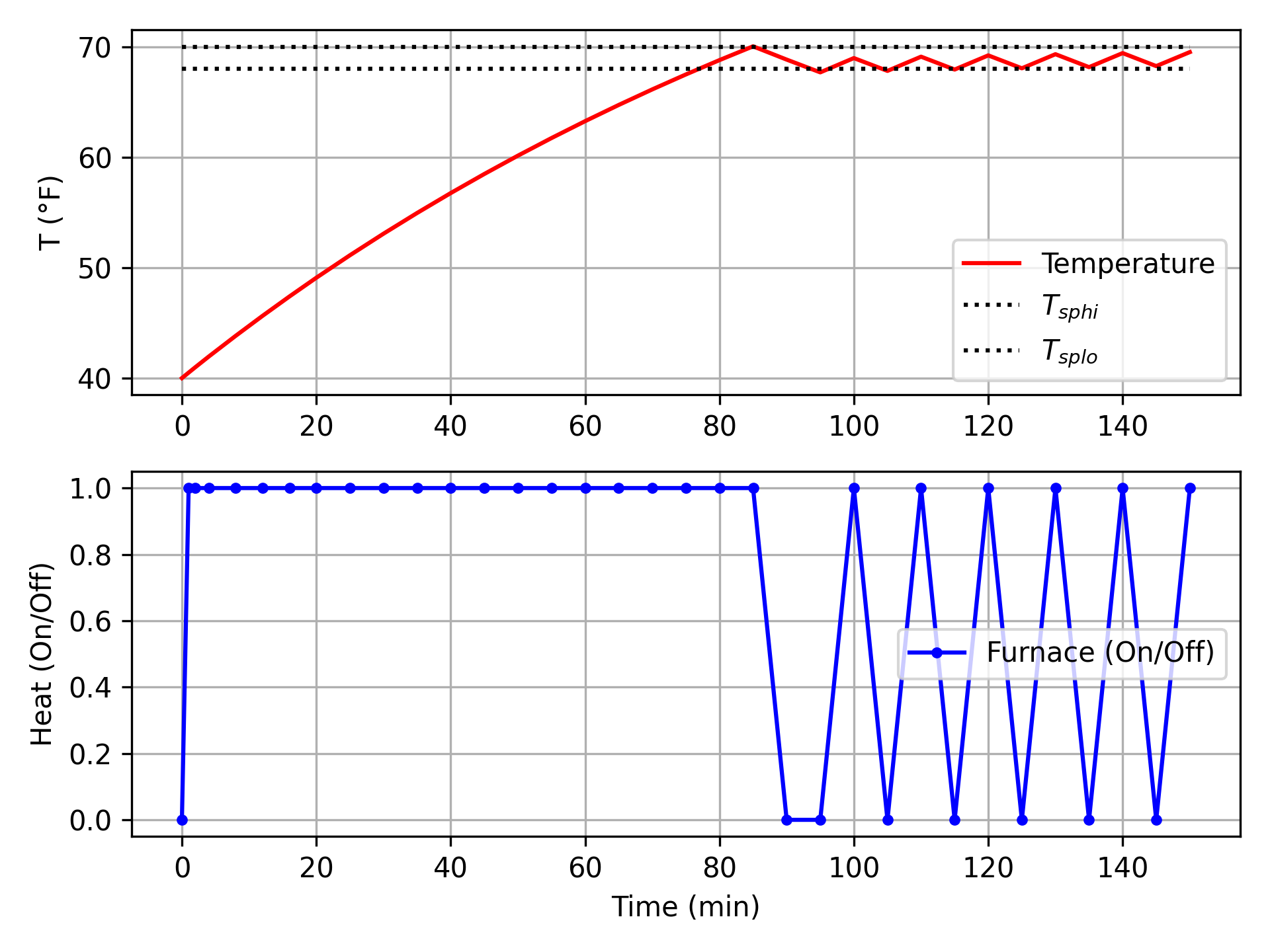
Design a thermostat for a home that has a furnace with On/Off control. The home is initially unheated in 40°F weather. When the heater is turned on, the temperature in the home reaches 63% of the steady state value in 120 minutes, starting from 40°F. If left on indefinitely, the home eventually reaches 100°F. Optimize the heater response for the first 2 1/2 hours starting from a cold home at 40°F. The target range for the home is between 68 and 70°F.

import matplotlib.pyplot as plt
m = GEKKO(remote=False) # create GEKKO model
m.time = [0,1,2,4,8,12,16,20,25,30,35,40,45,50,\
55,60,65,70,75,80,85,90,95,100,105,110,\
115,120,125,130,135,140,145,150]
# change solver options
m.solver_options = ['minlp_gap_tol 1.0e-2',\
'minlp_maximum_iterations 10000',\
'minlp_max_iter_with_int_sol 5000']
m.options.SOLVER = 1
m.options.IMODE = 6
# parameters
Kp = 60; taup = 120; T0 = 40
# create heater binary variable
u = m.MV(integer=True,lb=0,ub=1)
u.DCOST = 0.1; u.STATUS = 1
# controlled variable (temperature)
T = m.CV(value=T0)
T.SPHI = 70; T.SPLO = 68
T.STATUS = 1; T.TR_INIT = 0
# first order equation
m.Equation(taup * T.dt() == -(T-T0) + Kp * u)
m.solve() # solve MILP
# plot solution
plt.subplot(2,1,1)
plt.plot(m.time,T,'r-',label='Temperature')
plt.plot([0,m.time[-1]],[T.SPHI,T.SPHI],'k:',label=r'$T_{sphi}$')
plt.plot([0,m.time[-1]],[T.SPLO,T.SPLO],'k:',label=r'$T_{splo}$')
plt.ylabel('T (°F)'); plt.legend(), plt.grid()
plt.subplot(2,1,2)
plt.plot(m.time,u,'b.-',label='Furnace (On/Off)')
plt.ylabel('Heat (On/Off)'); plt.xlabel('Time (min)')
plt.legend(); plt.grid(); plt.tight_layout()
plt.savefig('furnace_control.png',dpi=300)
plt.show()


The Gekko Optimization Suite is a machine learning and optimization package in Python for mixed-integer and differential algebraic equations. The GEKKO package is available in Python with pip install gekko. There are additional example problems for equation solving, optimization, regression, dynamic simulation, model predictive control, and machine learning. Cite Gekko Paper
