Dynamic Optimization

        plt.plot(tm[0:i],Tsp1[0:i],'k-',lw=2,label=r'$T_1 SP$')

        plt.plot(tm[0:i],Tsp2[0:i],'g-',lw=2,label=r'$T_2 SP$')

        plt.plot(tm[0:i],Q1s[0:i],'r-',lw=3,label=r'$Q_1$')
        plt.plot(tm[0:i],Q2s[0:i],'b:',lw=3,label=r'$Q_2$')

        plt.plot(tm[0:i],T1sp[0:i],'k-',lw=2,label=r'$T_1 SP$')

        plt.plot(tm[0:i],T2sp[0:i],'g-',lw=2,label=r'$T_2 SP$')

        plt.plot(tm[0:i],Q1s[0:i],'r-',lw=3,label=r'$Q_1$')
        plt.plot(tm[0:i],Q2s[0:i],'b:',lw=3,label=r'$Q_2$')

Virtual TCLab on Google Colab

Tsp1[3:] = 40.0 Tsp2[40:] = 30.0 Tsp1[80:] = 32.0 Tsp2[120:] = 35.0 Tsp1[160:] = 45.0

        plt.plot(tm[0:i],Tsp1[0:i],'k-',LineWidth=2,label=r'$T_1 SP$')

        plt.plot(tm[0:i],Tsp2[0:i],'g-',LineWidth=2,label=r'$T_2 SP$')

        plt.plot(tm[0:i],T1sp[0:i],'k-',LineWidth=2,label=r'$T_1 SP$')

        plt.plot(tm[0:i],T2sp[0:i],'g-',LineWidth=2,label=r'$T_2 SP$')

• Steady state data set 1 (low power heaters)

url = 'https://apmonitor.com/do/uploads/Main/tclab_ss_data3.txt'

Training data is generated from the script in TCLab B or use one of the data files below.

• Steady state data set 1 (low power heaters)
• Steady state data set 2 (high power heaters)

url = 'https://apmonitor.com/do/uploads/Main/tclab_ss_data1.txt'

1. Initialize Model

1. Make sure serial connection still closes when there's an error

except:

    # Disconnect from Arduino
    a.Q1(0)
    a.Q2(0)
    print('Error: Shutting down')
    a.close()
    raise

(:sourceend:) (:divend:)

(:toggle hide gekko_labGNN button show="Lab G: Python TCLab MIMO MPC with Neural Network Model":) (:div id=gekko_labGNN:) (:source lang=python:) import numpy as np import pandas as pd import matplotlib.pyplot as plt from sklearn.preprocessing import MinMaxScaler from gekko import GEKKO import tclab import time

1. -------------------------------------
2. connect to Arduino
3. -------------------------------------

a = tclab.TCLab()

1. -------------------------------------
2. import data
3. -------------------------------------

url = 'https://apmonitor.com/do/uploads/Main/tclab_ss_data2.txt' data = pd.read_csv(url)

1. -------------------------------------
2. scale data
3. -------------------------------------

s = MinMaxScaler(feature_range=(0,1)) sc_train = s.fit_transform(data)

1. partition into inputs and outputs

xs = sc_train[:,0:2] # 2 heaters ys = sc_train[:,2:4] # 2 temperatures

1. -------------------------------------
2. build neural network
3. -------------------------------------

nin = 2 # inputs n1 = 2 # hidden layer 1 (linear) n2 = 2 # hidden layer 2 (nonlinear) n3 = 2 # hidden layer 3 (linear) nout = 2 # outputs

1. Initialize gekko models

train = GEKKO() mpc = GEKKO(remote=False) model = [train,mpc]

for m in model:

    # use APOPT solver
    m.options.SOLVER = 1

    # input(s)
    if m==train:
        # parameter for training
        m.inpt = [m.Param() for i in range(nin)]
    else:
        # variable for MPC
        m.inpt = [m.Var() for i in range(nin)]        

    # layer 1 (linear)
    m.w1 = m.Array(m.FV, (nout,nin,n1))
    m.l1 = [[m.Intermediate(sum([m.w1[k,j,i]*m.inpt[j]             for j in range(nin)])) for i in range(n1)]             for k in range(nout)]

    # layer 2 (tanh)
    m.w2 = m.Array(m.FV, (nout,n1,n2))
    m.l2 = [[m.Intermediate(sum([m.tanh(m.w2[k,j,i]*m.l1[k][j])             for j in range(n1)])) for i in range(n2)]             for k in range(nout)]

    # layer 3 (linear)
    m.w3 = m.Array(m.FV, (nout,n2,n3))
    m.l3 = [[m.Intermediate(sum([m.w3[k,j,i]*m.l2[k][j]             for j in range(n2)])) for i in range(n3)]             for k in range(nout)]

    # outputs
    m.outpt = [m.CV() for i in range(nout)]
    m.Equations([m.outpt[k]==sum([m.l3[k][i] for i in range(n3)])                  for k in range(nout)])

    # flatten matrices
    m.w1 = m.w1.flatten()
    m.w2 = m.w2.flatten()
    m.w3 = m.w3.flatten()

1. -------------------------------------
2. fit parameter weights
3. -------------------------------------

m = train for i in range(nin):

    m.inpt[i].value=xs[:,i]

for i in range(nout):

    m.outpt[i].value = ys[:,i]
    m.outpt[i].FSTATUS = 1

for i in range(len(m.w1)):

    m.w1[i].FSTATUS=1
    m.w1[i].STATUS=1
    m.w1[i].MEAS=1.0

for i in range(len(m.w2)):

    m.w2[i].STATUS=1
    m.w2[i].FSTATUS=1
    m.w2[i].MEAS=0.5

for i in range(len(m.w3)):

    m.w3[i].FSTATUS=1
    m.w3[i].STATUS=1
    m.w3[i].MEAS=1.0

m.options.IMODE = 2 m.options.EV_TYPE = 2

1. solve for weights to minimize loss (objective)

m.solve(disp=True)

1. -------------------------------------
2. Create Model Predictive Controller
3. -------------------------------------

m = mpc

1. 60 second time horizon, steps of 3 sec

m.time = np.linspace(0,60,21)

1. load neural network parameters

for i in range(len(m.w1)):

    m.w1[i].MEAS=train.w1[i].NEWVAL
    m.w1[i].FSTATUS = 1

for i in range(len(m.w2)):

    m.w2[i].MEAS=train.w2[i].NEWVAL
    m.w2[i].FSTATUS = 1

for i in range(len(m.w3)):

    m.w3[i].MEAS=train.w3[i].NEWVAL
    m.w3[i].FSTATUS = 1

1. MVs and CVs

Q1 = m.MV(value=0) Q2 = m.MV(value=0) TC1 = m.CV(value=a.T1) TC2 = m.CV(value=a.T2)

1. scaled inputs to neural network

m.Equation(m.inpt[0] == Q1 * s.scale_[0] + s.min_[0]) m.Equation(m.inpt[1] == Q2 * s.scale_[1] + s.min_[1])

1. define Temperature output

Q0 = 0 # initial heater T0 = 23 # ambient temperature

1. scaled steady state ouput

T1_ss = m.Var(value=T0) T2_ss = m.Var(value=T0) m.Equation(T1_ss == (m.outpt[0]-s.min_[2])/s.scale_[2]) m.Equation(T2_ss == (m.outpt[1]-s.min_[3])/s.scale_[3])

1. time constants

tauA = m.Param(value=80) tauB = m.Param(value=20) TH1 = m.Var(a.T1) TH2 = m.Var(a.T2)

1. additional model equation for dynamics

m.Equation(tauA*TH1.dt()==-TH1+T1_ss) m.Equation(tauA*TH2.dt()==-TH2+T2_ss) m.Equation(tauB*TC1.dt()==-TC1+TH1) m.Equation(tauB*TC2.dt()==-TC2+TH2)

1. Manipulated variable tuning

Q1.STATUS = 1 # use to control temperature Q1.FSTATUS = 0 # no feedback measurement Q1.LOWER = 0.0 Q1.UPPER = 100.0 Q1.DMAX = 40.0 Q1.COST = 0.0 Q1.DCOST = 0.0

Q2.STATUS = 1 # use to control temperature Q2.FSTATUS = 0 # no feedback measurement Q2.LOWER = 0.0 Q2.UPPER = 100.0 Q2.DMAX = 40.0 Q2.COST = 0.0 Q2.DCOST = 0.0

1. Controlled variable tuning

TC1.STATUS = 1 # minimize error with setpoint range TC1.FSTATUS = 1 # receive measurement TC1.TR_INIT = 1 # reference trajectory TC1.TAU = 10 # time constant for response

TC2.STATUS = 1 # minimize error with setpoint range TC2.FSTATUS = 1 # receive measurement TC2.TR_INIT = 1 # reference trajectory TC2.TAU = 10 # time constant for response

1. Global Options

m.options.IMODE = 6 # MPC m.options.CV_TYPE = 1 # Objective type m.options.NODES = 3 # Collocation nodes m.options.SOLVER = 3 # 1=APOPT, 3=IPOPT

1. -------------------------------------
2. Initialize model and data storage
3. -------------------------------------
4. Get Version

print(a.version)

1. Turn LED on

print('LED On') a.LED(100)

1. Run time in minutes

run_time = 10.0

1. Number of cycles with 3 second intervals

loops = int(20.0*run_time) tm = np.zeros(loops)

1. Temperature (K)

T1 = np.ones(loops) * a.T1 # temperature (degC) T1sp = np.ones(loops) * 35.0 # set point (degC) T2 = np.ones(loops) * a.T2 # temperature (degC) T2sp = np.ones(loops) * 23.0 # set point (degC)

1. Set point changes

T1sp[3:] = 40.0 T2sp[40:] = 30.0 T1sp[80:] = 32.0 T2sp[120:] = 35.0 T1sp[160:] = 45.0

1. heater values

Q1s = np.ones(loops) * 0.0 Q2s = np.ones(loops) * 0.0

1. Create plot

plt.figure() plt.ion() plt.show()

1. Main Loop

start_time = time.time() prev_time = start_time try:

    for i in range(1,loops):
        # Sleep time
        sleep_max = 3.0
        sleep = sleep_max - (time.time() - prev_time)
        if sleep>=0.01:
            time.sleep(sleep)
        else:
            time.sleep(0.01)

        # Record time and change in time
        t = time.time()
        dt = t - prev_time
        prev_time = t
        tm[i] = t - start_time

        # Read temperatures in Kelvin 
        T1[i] = a.T1
        T2[i] = a.T2

        ###############################
        ### MPC CONTROLLER          ###
        ###############################
        TC1.MEAS = T1[i]
        TC2.MEAS = T2[i]
        # input setpoint with deadband +/- DT
        DT = 0.1
        TC1.SPHI = T1sp[i] + DT
        TC1.SPLO = T1sp[i] - DT
        TC2.SPHI = T2sp[i] + DT
        TC2.SPLO = T2sp[i] - DT
        # solve MPC
        m.solve(disp=False)    
        # test for successful solution
        if (m.options.APPSTATUS==1):
            # retrieve the first Q value
            Q1s[i] = Q1.NEWVAL
            Q2s[i] = Q2.NEWVAL
        else:
            # not successful, set heater to zero
            Q1s[i] = 0        
            Q2s[i] = 0        

        # Write output (0-100)
        a.Q1(Q1s[i])
        a.Q2(Q2s[i])

        # Plot
        plt.clf()
        ax=plt.subplot(3,1,1)
        ax.grid()
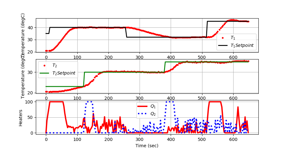
        plt.plot(tm[0:i],T1[0:i],'ro',MarkerSize=3,label=r'$T_1$')
        plt.plot(tm[0:i],T1sp[0:i],'k-',LineWidth=2,label=r'$T_1 Setpoint$')
        plt.ylabel('Temperature (degC)')
        plt.legend(loc='best')
        ax=plt.subplot(3,1,2)
        ax.grid()
        plt.plot(tm[0:i],T2[0:i],'ro',MarkerSize=3,label=r'$T_2$')
        plt.plot(tm[0:i],T2sp[0:i],'g-',LineWidth=2,label=r'$T_2 Setpoint$')
        plt.ylabel('Temperature (degC)')
        plt.legend(loc='best')
        ax=plt.subplot(3,1,3)
        ax.grid()
        plt.plot(tm[0:i],Q1s[0:i],'r-',LineWidth=3,label=r'$Q_1$')
        plt.plot(tm[0:i],Q2s[0:i],'b:',LineWidth=3,label=r'$Q_2$')
        plt.ylabel('Heaters')
        plt.xlabel('Time (sec)')
        plt.legend(loc='best')
        plt.draw()
        plt.pause(0.05)

    # Turn off heaters
    a.Q1(0)
    a.Q2(0)
    print('Shutting down') 

1. Allow user to end loop with Ctrl-C

except KeyboardInterrupt:

    # Disconnect from Arduino
    a.Q1(0)
    a.Q2(0)
    print('Shutting down')
    a.close()

import tclab

a = tclab.TCLab()

1. Get Version

print(a.version)

1. Turn LED on

print('LED On') a.LED(100)

1. Run time in minutes

run_time = 10.0

1. Number of cycles with 3 second intervals

loops = int(20.0*run_time) tm = np.zeros(loops)

1. Temperature (K)

T1 = np.ones(loops) * a.T1 # temperature (degC) Tsp1 = np.ones(loops) * 35.0 # set point (degC) T2 = np.ones(loops) * a.T2 # temperature (degC) Tsp2 = np.ones(loops) * 23.0 # set point (degC)

1. Set point changes

1. heater values

Q1s = np.ones(loops) * 0.0 Q2s = np.ones(loops) * 0.0

1. remote=True for MacOS

1. 60 second time horizon, steps of 3 sec

m.time = np.linspace(0,60,21)

1. Parameters

U = m.FV(value=10,name='u') tau = m.FV(value=5,name='tau') alpha1 = m.FV(value=0.01) # W / % heater alpha2 = m.FV(value=0.0075) # W / % heater

Kp = m.Param(value=0.5) tau = m.Param(value=50.0) zeta = m.Param(value=1.5)

1. Manipulated variables

Q1.STATUS = 1 # use to control temperature Q1.FSTATUS = 0 # no feedback measurement

Q1.UPPER = 100.0 Q1.DMAX = 40.0 Q1.COST = 0.0 Q1.DCOST = 0.0

Q2.STATUS = 1 # use to control temperature Q2.FSTATUS = 0 # no feedback measurement

Q2.UPPER = 100.0 Q2.DMAX = 40.0 Q2.COST = 0.0 Q2.DCOST = 0.0

1. Controlled variable

TC1 = m.CV(value=T1[0]) TC1.STATUS = 1 # minimize error with setpoint range

TC1.TR_INIT = 1 # reference trajectory TC1.TAU = 10 # time constant for response

1. Controlled variable

TC2 = m.CV(value=T2[0]) TC2.STATUS = 1 # minimize error with setpoint range

TC2.TR_INIT = 1 # reference trajectory TC2.TAU = 10 # time constant for response

1. State variables

TH1 = m.SV(value=T1[0]) TH2 = m.SV(value=T2[0])

Ta = m.Param(value=23.0+273.15) # K mass = m.Param(value=4.0/1000.0) # kg Cp = m.Param(value=0.5*1000.0) # J/kg-K A = m.Param(value=10.0/100.0**2) # Area not between heaters in m^2 As = m.Param(value=2.0/100.0**2) # Area between heaters in m^2 eps = m.Param(value=0.9) # Emissivity sigma = m.Const(5.67e-8) # Stefan-Boltzmann

1. Heater temperatures

T1i = m.Intermediate(TH1+273.15) T2i = m.Intermediate(TH2+273.15)

Q_C12 = m.Intermediate(U*As*(T2i-T1i)) # Convective Q_R12 = m.Intermediate(eps*sigma*As*(T2i**4-T1i**4)) # Radiative

1. Semi-fundamental correlations (energy balances)

m.Equation(TH1.dt() == (1.0/(mass*Cp))*(U*A*(Ta-T1i) + eps * sigma * A * (Ta**4 - T1i**4) + Q_C12 + Q_R12 + alpha1*Q1))

m.Equation(TH2.dt() == (1.0/(mass*Cp))*(U*A*(Ta-T2i) + eps * sigma * A * (Ta**4 - T2i**4) - Q_C12 - Q_R12 + alpha2*Q2))

1. Empirical correlations (lag equations to emulate conduction)

m.Equation(tau * TC1.dt() == -TC1 + TH1) m.Equation(tau * TC2.dt() == -TC2 + TH2)

m.options.IMODE = 6 # MPC m.options.CV_TYPE = 1 # Objective type

m.options.SOLVER = 3 # 1=APOPT, 3=IPOPT

plt.figure()

    for i in range(1,loops):

            time.sleep(sleep)

        # Read temperatures in Kelvin 
        T1[i] = a.T1
        T2[i] = a.T2

        ###############################
        ### MPC CONTROLLER          ###
        ###############################
        TC1.MEAS = T1[i]
        TC2.MEAS = T2[i]
        # input setpoint with deadband +/- DT
        DT = 0.1
        TC1.SPHI = Tsp1[i] + DT
        TC1.SPLO = Tsp1[i] - DT
        TC2.SPHI = Tsp2[i] + DT
        TC2.SPLO = Tsp2[i] - DT
        # solve MPC
        m.solve(disp=False)    
        # test for successful solution
        if (m.options.APPSTATUS==1):
            # retrieve the first Q value
            Q1s[i] = Q1.NEWVAL
            Q2s[i] = Q2.NEWVAL
        else:
            # not successful, set heater to zero
            Q1s[i] = 0        
            Q2s[i] = 0        

        # Write output (0-100)

        ax=plt.subplot(3,1,1)

        plt.plot(tm[0:i],T1[0:i],'ro',MarkerSize=3,label=r'$T_1$')
        plt.plot(tm[0:i],Tsp1[0:i],'k-',LineWidth=2,label=r'$T_1 Setpoint$')

        plt.legend(loc='best')
        ax=plt.subplot(3,1,2)

        plt.plot(tm[0:i],T2[0:i],'ro',MarkerSize=3,label=r'$T_2$')
        plt.plot(tm[0:i],Tsp2[0:i],'g-',LineWidth=2,label=r'$T_2 Setpoint$')
        plt.ylabel('Temperature (degC)')

        ax=plt.subplot(3,1,3)
        ax.grid()
        plt.plot(tm[0:i],Q1s[0:i],'r-',LineWidth=3,label=r'$Q_1$')
        plt.plot(tm[0:i],Q2s[0:i],'b:',LineWidth=3,label=r'$Q_2$')
        plt.ylabel('Heaters')
        plt.xlabel('Time (sec)')
        plt.legend(loc='best')

    # Turn off heaters

    print('Shutting down') 

    # Disconnect from Arduino

    print('Shutting down')

    print('Error: Shutting down')

(:title TCLab G - Nonlinear MPC:)

(:title TCLab G - Nonlinear Model Predictive Control:) (:keywords Arduino, Empirical, Hybrid, MPC, Regression, temperature, control, process control, course:) (:description Nonlinear Model Predictive Control for Temperature Control with Arduino Temperature Sensors and Heaters in MATLAB and Python:)

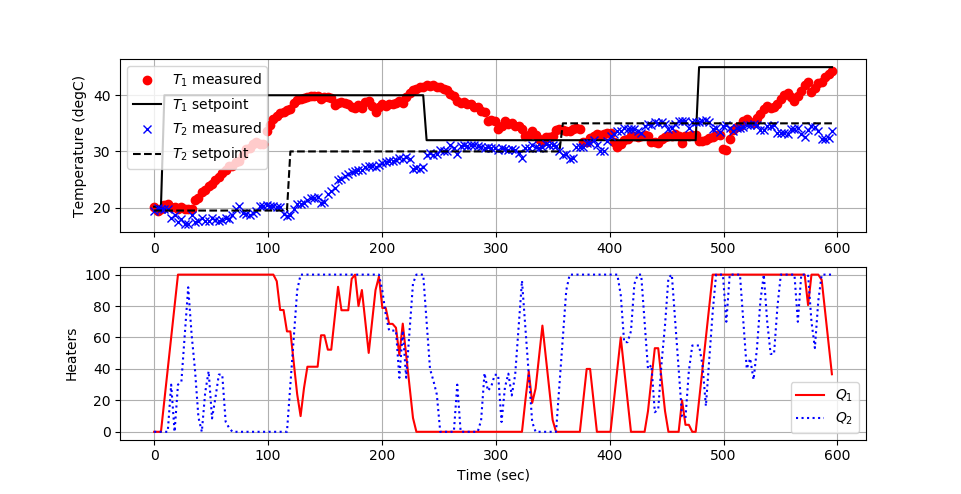
The TCLab is a hands-on application of machine learning and advanced temperature control with two heaters and two temperature sensors. The labs reinforce principles of model development, estimation, and advanced control methods. This is the seventh exercise and it involves nonlinear model predictive control with an energy balance model that is augmented with empirical elements. The predictions were previously aligned to the measured values through an estimator. This model predictive controller uses those parameters and a nonlinear MIMO (Multiple Input, Multiple Output) model of the TCLab input to output response to control temperatures to a set point.

Lab Problem Statement

• Lab G - Nonlinear Model Predictive Control

Data and Solutions

• Solution with MATLAB and Python

(:html:) <iframe width="560" height="315" src="https://www.youtube.com/embed/eoZRcbilKTU" frameborder="0" allow="accelerometer; autoplay; encrypted-media; gyroscope; picture-in-picture" allowfullscreen></iframe> (:htmlend:)

(:toggle hide gekko_labG button show="Lab G: Python TCLab MIMO MPC with Hybrid Model":) (:div id=gekko_labG:) (:source lang=python:) import numpy as np import time import matplotlib.pyplot as plt import random

1. get gekko package with:
2. pip install gekko

from gekko import GEKKO

1. get tclab package with:
2. pip install tclab

from tclab import TCLab

1. Connect to Arduino

a = TCLab()

1. Final time

tf = 10 # min

1. number of data points (every 3 seconds)

n = tf * 20 + 1

1. Percent Heater (0-100%)

Q1s = np.zeros(n) Q2s = np.zeros(n)

1. Temperatures (degC)

T1m = a.T1 * np.ones(n) T2m = a.T2 * np.ones(n)

1. Temperature setpoints

T1sp = T1m[0] * np.ones(n) T2sp = T2m[0] * np.ones(n)

1. Heater set point steps about every 150 sec

T1sp[3:] = 40.0 T2sp[40:] = 30.0 T1sp[80:] = 32.0 T2sp[120:] = 35.0 T1sp[160:] = 45.0

1. Initialize Model as Estimator

2. use remote=True for MacOS

m = GEKKO(name='tclab-mpc',remote=False)

1. Control horizon, non-uniform time steps

m.time = [0,3,6,10,14,18,22,27,32,38,45,55,65, 75,90,110,130,150]

1. Parameters from Estimation

K1 = m.FV(value=0.607) K2 = m.FV(value=0.293) K3 = m.FV(value=0.24) tau12 = m.FV(value=192) tau3 = m.FV(value=15)

1. don't update parameters with optimizer

K1.STATUS = 0 K2.STATUS = 0 K3.STATUS = 0 tau12.STATUS = 0 tau3.STATUS = 0

1. Measured inputs

Q1 = m.MV(value=0) Q1.STATUS = 1 # manipulated Q1.FSTATUS = 0 # measured Q1.DMAX = 20.0 Q1.DCOST = 0.1 Q1.UPPER = 100.0 Q1.LOWER = 0.0

Q2 = m.MV(value=0) Q2.STATUS = 1 # manipulated Q2.FSTATUS = 0 # measured Q2.DMAX = 30.0 Q2.DCOST = 0.1 Q2.UPPER = 100.0 Q2.LOWER = 0.0

1. State variables

TH1 = m.SV(value=T1m[0]) TH2 = m.SV(value=T2m[0])

1. Measurements for model alignment

TC1 = m.CV(value=T1m[0]) TC1.STATUS = 1 # minimize error TC1.FSTATUS = 1 # receive measurement TC1.TAU = 10 # response speed (time constant) TC1.TR_INIT = 2 # reference trajectory

TC2 = m.CV(value=T2m[0]) TC2.STATUS = 1 # minimize error TC2.FSTATUS = 1 # receive measurement TC2.TAU = 10 # response speed (time constant) TC2.TR_INIT = 2 # reference trajectory

Ta = m.Param(value=23.0) # degC

1. Heat transfer between two heaters

DT = m.Intermediate(TH2-TH1)

1. Empirical correlations

m.Equation(tau12 * TH1.dt() + (TH1-Ta) == K1*Q1 + K3*DT) m.Equation(tau12 * TH2.dt() + (TH2-Ta) == K2*Q2 - K3*DT) m.Equation(tau3 * TC1.dt() + TC1 == TH1) m.Equation(tau3 * TC2.dt() + TC2 == TH2)

1. Global Options

m.options.IMODE = 6 # MHE m.options.EV_TYPE = 1 # Objective type m.options.NODES = 3 # Collocation nodes m.options.SOLVER = 3 # IPOPT m.options.COLDSTART = 1 # COLDSTART on first cycle

1. Create plot

plt.figure(figsize=(10,7)) plt.ion() plt.show()

1. Main Loop

start_time = time.time() prev_time = start_time tm = np.zeros(n)

try:

    for i in range(1,n):
        # Sleep time
        sleep_max = 3.0
        sleep = sleep_max - (time.time() - prev_time)
        if sleep>=0.01:
            time.sleep(sleep-0.01)
        else:
            time.sleep(0.01)

        # Record time and change in time
        t = time.time()
        dt = t - prev_time
        prev_time = t
        tm[i] = t - start_time

        # Read temperatures in Celsius 
        T1m[i] = a.T1
        T2m[i] = a.T2

        # Insert measurements
        TC1.MEAS = T1m[i]
        TC2.MEAS = T2m[i]

        # Adjust setpoints
        TC1.SPHI = T1sp[i] + 0.1
        TC1.SPLO = T1sp[i] - 0.1

        TC2.SPHI = T2sp[i] + 0.1
        TC2.SPLO = T2sp[i] - 0.1

        # Predict Parameters and Temperatures with MHE
        # use remote=False for local solve
        m.solve() 

        if m.options.APPSTATUS == 1:
            # Retrieve new values
            Q1s[i]  = Q1.NEWVAL
            Q2s[i]  = Q2.NEWVAL
        else:
            # Solution failed
            Q1s[i]  = 0.0
            Q2s[i]  = 0.0

        # Write new heater values (0-100)
        a.Q1(Q1s[i])
        a.Q2(Q2s[i])

        # Plot
        plt.clf()
        ax=plt.subplot(2,1,1)
        ax.grid()
        plt.plot(tm[0:i],T1m[0:i],'ro',label=r'$T_1$ measured')
        plt.plot(tm[0:i],T1sp[0:i],'k-',label=r'$T_1$ setpoint')
        plt.plot(tm[0:i],T2m[0:i],'bx',label=r'$T_2$ measured')
        plt.plot(tm[0:i],T2sp[0:i],'k--',label=r'$T_2$ setpoint')
        plt.ylabel('Temperature (degC)')
        plt.legend(loc=2)
        ax=plt.subplot(2,1,2)
        ax.grid()
        plt.plot(tm[0:i],Q1s[0:i],'r-',label=r'$Q_1$')
        plt.plot(tm[0:i],Q2s[0:i],'b:',label=r'$Q_2$')
        plt.ylabel('Heaters')
        plt.xlabel('Time (sec)')
        plt.legend(loc='best')
        plt.draw()
        plt.pause(0.05)

    # Turn off heaters and close connection
    a.Q1(0)
    a.Q2(0)
    a.close()
    # Save figure
    plt.savefig('tclab_mpc.png')

1. Allow user to end loop with Ctrl-C

except KeyboardInterrupt:

    # Turn off heaters and close connection
    a.Q1(0)
    a.Q2(0)
    a.close()
    print('Shutting down')
    plt.savefig('tclab_mpc.png')

1. Make sure serial connection still closes when there's an error

except:

    # Disconnect from Arduino
    a.Q1(0)
    a.Q2(0)
    a.close()
    print('Error: Shutting down')
    plt.savefig('tclab_mpc.png')
    raise

(:sourceend:) (:divend:)

See also:

Advanced Control Lab Overview

GEKKO Documentation

TCLab Documentation

TCLab Files on GitHub

Basic (PID) Control Lab

(:html:) <style> .button {

  border-radius: 4px;
  background-color: #0000ff;
  border: none;
  color: #FFFFFF;
  text-align: center;
  font-size: 28px;
  padding: 20px;
  width: 300px;
  transition: all 0.5s;
  cursor: pointer;
  margin: 5px;

}

.button span {

  cursor: pointer;
  display: inline-block;
  position: relative;
  transition: 0.5s;

}

.button span:after {

  content: '\00bb';
  position: absolute;
  opacity: 0;
  top: 0;
  right: -20px;
  transition: 0.5s;

}

.button:hover span {

  padding-right: 25px;

}

.button:hover span:after {

  opacity: 1;
  right: 0;

} </style> (:htmlend:)