Dynamic Optimization

Hybrid Model Development

$$\tau \frac{dT_{c1}}{dt} = -T_{c1} + T_{h1}, \quad \tau \frac{dT_{c2}}{dt} = -T_{c2} + T_{h2}$$

MHE optimizes the parameters (U, `\tau`, `\alpha_1`, `\alpha_2`) to minimize the estimation error while maintaining physically meaningful constraints.

Case Study: TCLab Hybrid Model Estimation

The Temperature Control Lab (TCLab) is an Arduino-based system with two heaters and temperature sensors, providing a controlled environment for testing estimation and control algorithms. In this case study, a hybrid model is developed, integrating an energy balance formulation with empirical lag dynamics to better capture system behavior. Moving Horizon Estimation is employed to fine-tune key parameters, ensuring that the model predictions closely align with measured data.

Mathematical Formulation for Hybrid Model Estimation

The TCLab hybrid model consists of four ordinary differential equations describing the heater and sensor temperatures. The energy balance equations for the heaters are:

$$m C_p \frac{dT_{h1}}{dt} = U A (T_{\infty} - T_{h1}) + \epsilon \sigma A (T_{\infty}^4 - T_{h1}^4) + \alpha_1 Q_1$$

$$m C_p \frac{dT_{h2}}{dt} = U A (T_{\infty} - T_{h2}) + \epsilon \sigma A (T_{\infty}^4 - T_{h2}^4) + \alpha_2 Q_2$$

where $T_{\infty}$ represents ambient temperature, $U$ is the heat transfer coefficient, and $\alpha_1,\alpha_2$ are heater power-to-heat conversion factors. To account for sensor delays, additional empirical lag equations are introduced:

$$\tau \frac{dT_{c1}}{dt} = -T_{c1} + T_{h1}, \quad \t\tau \frac{dT_{c2}}{dt} = -T_{c2} + T_{h2}$$

MHE optimizes the parameters $(U, \tau, \alpha_1, \alpha_2)$ to minimize the estimation error while maintaining physically meaningful constraints.

Python Implementation of MHE

The estimation framework is implemented using the GEKKO library in Python. The process involves defining system equations, incorporating measurement data, configuring solver settings, and iteratively updating estimates. The sliding horizon approach continuously updates state and parameter estimates as new data become available, ensuring real-time adaptability.

Results and Interpretation

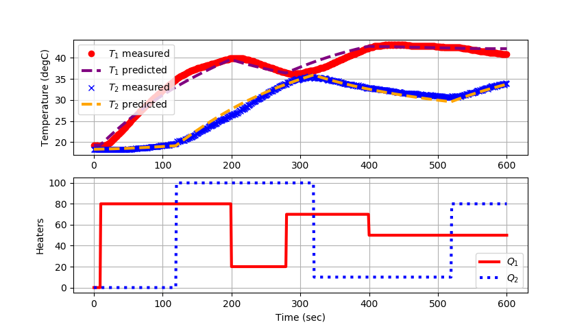
Applying MHE to TCLab data results in agreement between predicted and measured temperatures. The hybrid model successfully captures both fast and slow thermal responses. Estimated parameters, including heat transfer coefficients and lag constants, converge to stable and physically meaningful values. The choice between L1 and L2 norms in the objective function influences noise sensitivity, with L1 providing superior robustness to outliers.

Challenges in Estimation and Hybrid Modeling

Despite their advantages, estimation methods face challenges such as handling noisy data, computational complexity, and ensuring real-time performance. MHE and Bayesian methods require significant processing power, making them less feasible for high-speed applications without optimization techniques. Model uncertainty remains a key issue, as estimators are only as accurate as the models they rely on. Careful model selection, robust tuning, and noise rejection strategies are necessary to achieve reliable estimation.

Estimation Research

Emerging research in estimation focuses on integrating machine learning with traditional methods. Learning-based Kalman filters, hybrid models with adaptive online learning, and uncertainty-aware Bayesian estimators are gaining attention. Improved solver efficiency and distributed estimation techniques enable applications in large-scale systems such as industrial automation and autonomous robotics. Future estimators will likely leverage deep learning and probabilistic modeling to enhance robustness and adaptability.

Conclusion

Estimation is a cornerstone of control and optimization, enabling real-time decision-making based on incomplete information. The choice of estimation technique depends on computational constraints, system complexity, and noise characteristics. Hybrid modeling offers a promising avenue for improving estimation accuracy by integrating physics-based and data-driven methods. As research advances, estimation frameworks will continue to evolve, incorporating learning-based adaptations and advanced uncertainty quantification techniques to enhance applicability in real-world systems.

Estimation is the process of inferring internal states or parameters of a dynamic system using limited measurements and a model. This is essential in control applications, where direct measurement of all states is often impractical. By fusing models with sensor data, estimation provides the best possible approximation of the system's true state. However, estimation is not without its challenges. Noise in measurements, uncertainty in models, nonlinear system dynamics, and constraints on states complicate the task of designing robust and reliable estimators.

Dynamic Estimation Objectives

At the core of estimation lies the definition of an objective function that quantifies the discrepancy between model predictions and actual measurements. A common choice is the sum of squared errors, represented mathematically as `J_{2}=\sum (y_{\text{meas}}-y_{\text{pred}})^2`. This formulation is widely used due to its differentiability, which simplifies optimization. Alternatively, the sum of absolute errors (L1-norm), `J_{1}=\sum |y_{\text{meas}}-y_{\text{pred}}|`, is preferred in applications requiring robustness against outliers. The general optimization formulation for dynamic estimation is given by:

$$\min_{\hat{x}(0..N)} \sum_{k=0}^{N} \|y_k - h(\hat{x}_k)\|^p$$

subject to the system dynamics `\hat{x}_{k+1} = f(\hat{x}_k, u_k) ` and constraints that enforce physical feasibility. The choice of objective function impacts estimation accuracy and computational efficiency, influencing how well the estimator can reject noise and adapt to changing conditions.

Overview of Estimation Methods

Several approaches exist for state and parameter estimation. Moving Horizon Estimation (MHE) is an optimization-based technique that processes a sliding window of past data to estimate current states and parameters while incorporating constraints. The Kalman Filter (KF) is a recursive estimator that provides optimal state estimates for linear systems under Gaussian noise assumptions. Bayesian estimation methods, such as particle filters, explicitly apply Bayes' theorem to maintain probability distributions over states rather than single estimates. Least Squares (LS) estimation, particularly in its recursive form, is widely used for parameter identification and system modeling.

Comparison of Estimation Methods

The choice of estimation method depends on the problem at hand. The Kalman filter is computationally efficient but assumes linearity and Gaussian noise, making it less suitable for highly nonlinear systems. MHE, while more computationally demanding, naturally incorporates constraints and nonlinearity, often leading to superior accuracy in complex systems. Bayesian methods such as particle filters can handle non-Gaussian noise and multi-modal distributions but require significant computational resources. Least Squares estimation is effective for batch processing but lacks the adaptability needed for real-time applications.

Hybrid Model Development

Hybrid modeling combines physics-based first-principles equations with empirical data-driven corrections. This approach leverages known physical laws to ensure consistency while incorporating empirical elements to enhance accuracy. Hybrid models are particularly useful when the available physical models are incomplete or when data-driven techniques alone fail to generalize beyond the training set. Examples of hybrid modeling applications include climate simulations, manufacturing process control, and robotics, where physics-based constraints and data-driven flexibility are both required.

         lw=3,label=r'$T_1$ sensor')

         lw=3,label=r'$T_2$ sensor')

         lw=3,label=r'$Q_1$')

         lw=3,label=r'$Q_2$')

Virtual TCLab on Google Colab

Note: Switch to make_mp4 = True to make an MP4 movie animation. This requires imageio and ffmpeg (install available through Python). It creates a folder named figures in your run directory. You can delete this folder after the run is complete.

1. Make an MP4 animation?

make_mp4 = False if make_mp4:

    import imageio  # required to make animation
    import os
    try:
        os.mkdir('./figures')
    except:
        pass

1. change to remote=True for MacOS

tau = m.FV(value=5,name='tau')

tau.LOWER = 4 tau.UPPER = 8

        m.solve(disp=True) 

        if make_mp4:
            filename='./figures/plot_str(i+10000).png'
            plt.savefig(filename)

    # generate mp4 from png figures in batches of 350
    if make_mp4:
        images = []
        iset = 0
        for i in range(1,n):
            filename='./figures/plot_str(i+10000).png'
            images.append(imageio.imread(filename))
            if ((i+1)%350)==0:
                imageio.mimsave('results_str(iset).mp4', images)
                iset += 1
                images = []
        if images!=[]:
            imageio.mimsave('results_str(iset).mp4', images)

(:toggle hide gekko_labEm button show="Lab E: Python GEKKO Moving Horizon Estimation":) (:div id=gekko_labEm:)

import numpy as np import time import matplotlib.pyplot as plt import random

1. get gekko package with:
2. pip install gekko

from gekko import GEKKO

1. get tclab package with:
2. pip install tclab

from tclab import TCLab

1. Connect to Arduino

a = TCLab()

1. Final time

tf = 10 # min

1. number of data points (1 pt every 3 seconds)

n = tf * 20 + 1

1. Configure heater levels
2. Percent Heater (0-100%)

Q1s = np.zeros(n) Q2s = np.zeros(n)

1. Heater random steps every 50 sec
2. Alternate steps by Q1 and Q2

Q1s[3:] = 100.0 Q1s[50:] = 0.0 Q1s[100:] = 80.0

Q2s[25:] = 60.0 Q2s[75:] = 100.0 Q2s[125:] = 25.0

1. rapid, random changes every 5 cycles between 50 and 100

for i in range(130,180):

    if i%10==0:
        Q1s[i:i+10] = random.random() * 100.0
    if (i+5)%10==0:
        Q2s[i:i+10] = random.random() * 100.0

1. Record initial temperatures (degC)

T1m = a.T1 * np.ones(n) T2m = a.T2 * np.ones(n)

1. Store MHE values for plots

Tmhe1 = T1m[0] * np.ones(n) Tmhe2 = T2m[0] * np.ones(n) Umhe = 10.0 * np.ones(n) taumhe = 5.0 * np.ones(n) amhe1 = 0.01 * np.ones(n) amhe2 = 0.0075 * np.ones(n)

1. Initialize Model as Estimator

2. Use remote=False for local solve (Windows, Linux, ARM)
3. remote=True for remote solve (All platforms)

m = GEKKO(name='tclab-mhe',remote=False)

1. 60 second time horizon, 20 steps

m.time = np.linspace(0,60,21)

1. Parameters to Estimate

U = m.FV(value=10,name='u') U.STATUS = 0 # don't estimate initially U.FSTATUS = 0 # no measurements U.DMAX = 1 U.LOWER = 5 U.UPPER = 15

tau = m.FV(value=20,name='tau') tau.STATUS = 0 # don't estimate initially tau.FSTATUS = 0 # no measurements tau.DMAX = 1 tau.LOWER = 15 tau.UPPER = 25

alpha1 = m.FV(value=0.01,name='a1') # W / % heater alpha1.STATUS = 0 # don't estimate initially alpha1.FSTATUS = 0 # no measurements alpha1.DMAX = 0.001 alpha1.LOWER = 0.003 alpha1.UPPER = 0.03

alpha2 = m.FV(value=0.0075,name='a2') # W / % heater alpha2.STATUS = 0 # don't estimate initially alpha2.FSTATUS = 0 # no measurements alpha2.DMAX = 0.001 alpha2.LOWER = 0.002 alpha2.UPPER = 0.02

1. Measured inputs

Q1 = m.MV(value=0,name='q1') Q1.STATUS = 0 # don't estimate Q1.FSTATUS = 1 # receive measurement

Q2 = m.MV(value=0,name='q2') Q2.STATUS = 0 # don't estimate Q2.FSTATUS = 1 # receive measurement

1. State variables

TH1 = m.SV(value=T1m[0],name='th1') TH2 = m.SV(value=T2m[0],name='th2')

1. Measurements for model alignment

TC1 = m.CV(value=T1m[0],name='tc1') TC1.STATUS = 1 # minimize error between simulation and measurement TC1.FSTATUS = 1 # receive measurement TC1.MEAS_GAP = 0.1 # measurement deadband gap TC1.LOWER = 0 TC1.UPPER = 200

TC2 = m.CV(value=T2m[0],name='tc2') TC2.STATUS = 1 # minimize error between simulation and measurement TC2.FSTATUS = 1 # receive measurement TC2.MEAS_GAP = 0.1 # measurement deadband gap TC2.LOWER = 0 TC2.UPPER = 200

Ta = m.Param(value=23.0+273.15) # K mass = m.Param(value=4.0/1000.0) # kg Cp = m.Param(value=0.5*1000.0) # J/kg-K A = m.Param(value=10.0/100.0**2) # Area not between heaters in m^2 As = m.Param(value=2.0/100.0**2) # Area between heaters in m^2 eps = m.Param(value=0.9) # Emissivity sigma = m.Const(5.67e-8) # Stefan-Boltzmann

1. Heater temperatures

T1 = m.Intermediate(TH1+273.15) T2 = m.Intermediate(TH2+273.15)

1. Heat transfer between two heaters

Q_C12 = m.Intermediate(U*As*(T2-T1)) # Convective Q_R12 = m.Intermediate(eps*sigma*As*(T2**4-T1**4)) # Radiative

1. Semi-fundamental correlations (energy balances)

m.Equation(TH1.dt() == (1.0/(mass*Cp))*(U*A*(Ta-T1) + eps * sigma * A * (Ta**4 - T1**4) + Q_C12 + Q_R12 + alpha1*Q1))

m.Equation(TH2.dt() == (1.0/(mass*Cp))*(U*A*(Ta-T2) + eps * sigma * A * (Ta**4 - T2**4) - Q_C12 - Q_R12 + alpha2*Q2))

1. Empirical correlations (lag equations to emulate conduction)

m.Equation(tau * TC1.dt() == -TC1 + TH1) m.Equation(tau * TC2.dt() == -TC2 + TH2)

1. Global Options

m.options.IMODE = 5 # MHE m.options.EV_TYPE = 2 # Objective type m.options.NODES = 3 # Collocation nodes m.options.SOLVER = 3 # IPOPT m.options.COLDSTART = 1 # COLDSTART on first cycle

1. Create plot

plt.figure(figsize=(10,7)) plt.ion() plt.show()

1. Main Loop

start_time = time.time() prev_time = start_time tm = np.zeros(n)

try:

    for i in range(1,n):
        # Sleep time
        sleep_max = 3.0
        sleep = sleep_max - (time.time() - prev_time)
        if sleep>=0.01:
            time.sleep(sleep-0.01)
        else:
            time.sleep(0.01)

        # Record time and change in time
        t = time.time()
        dt = t - prev_time
        prev_time = t
        tm[i] = t - start_time

        # Read temperatures in Celsius 
        T1m[i] = a.T1
        T2m[i] = a.T2

        # Insert measurements
        TC1.MEAS = T1m[i]
        TC2.MEAS = T2m[i]
        Q1.MEAS = Q1s[i-1]
        Q2.MEAS = Q2s[i-1]

        # Start estimating U after 10 cycles (20 sec)
        if i==10:
            U.STATUS = 1
            tau.STATUS = 1
            alpha1.STATUS = 1
            alpha2.STATUS = 1

        # Predict Parameters and Temperatures with MHE
        m.solve() 

        if m.options.APPSTATUS == 1:
            # Retrieve new values
            Tmhe1[i] = TC1.MODEL
            Tmhe2[i] = TC2.MODEL
            Umhe[i]  = U.NEWVAL
            taumhe[i] = tau.NEWVAL
            amhe1[i] = alpha1.NEWVAL
            amhe2[i] = alpha2.NEWVAL
        else:
            # Solution failed, copy prior solution
            Tmhe1[i] = Tmhe1[i-1]
            Tmhe2[i] = Tmhe1[i-1]
            Umhe[i]  = Umhe[i-1]
            taumhe[i] = taumhe[i-1]
            amhe1[i] = amhe1[i-1]
            amhe2[i] = amhe2[i-1]

        # Write new heater values (0-100)
        a.Q1(Q1s[i])
        a.Q2(Q2s[i])

        # Plot
        plt.clf()
        ax=plt.subplot(3,1,1)
        ax.grid()
        plt.plot(tm[0:i],T1m[0:i],'ro',label=r'$T_1$ measured')
        plt.plot(tm[0:i],Tmhe1[0:i],'k-',label=r'$T_1$ MHE')
        plt.plot(tm[0:i],T2m[0:i],'bx',label=r'$T_2$ measured')
        plt.plot(tm[0:i],Tmhe2[0:i],'k--',label=r'$T_2$ MHE')
        plt.ylabel('Temperature (degC)')
        plt.legend(loc=2)
        ax=plt.subplot(3,1,2)
        ax.grid()
        plt.plot(tm[0:i],Umhe[0:i],'k-',label='Heat Transfer Coeff')
        plt.plot(tm[0:i],taumhe[0:i],'g:',label='Time Constant')        
        plt.plot(tm[0:i],amhe1[0:i]*1000,'r--',label=r'$\alpha_1$x1000')
        plt.plot(tm[0:i],amhe2[0:i]*1000,'b--',label=r'$\alpha_2$x1000')
        plt.ylabel('Parameters')
        plt.legend(loc='best')
        ax=plt.subplot(3,1,3)
        ax.grid()
        plt.plot(tm[0:i],Q1s[0:i],'r-',label=r'$Q_1$')
        plt.plot(tm[0:i],Q2s[0:i],'b:',label=r'$Q_2$')
        plt.ylabel('Heaters')
        plt.xlabel('Time (sec)')
        plt.legend(loc='best')
        plt.draw()
        plt.pause(0.05)

    # Turn off heaters
    a.Q1(0)
    a.Q2(0)
    # Save figure
    plt.savefig('tclab_mhe.png')

1. Allow user to end loop with Ctrl-C

except KeyboardInterrupt:

    # Disconnect from Arduino
    a.Q1(0)
    a.Q2(0)
    print('Shutting down')
    a.close()
    plt.savefig('tclab_mhe.png')

1. Make sure serial connection still closes when there's an error

except:

    # Disconnect from Arduino
    a.Q1(0)
    a.Q2(0)
    print('Error: Shutting down')
    a.close()
    plt.savefig('tclab_mhe.png')
    raise

import numpy as np import matplotlib.pyplot as plt import pandas as pd from gekko import GEKKO

1. Import or generate data

filename = 'tclab_dyn_data2.csv' try:

    data = pd.read_csv(filename)

except:

    url = 'https://apmonitor.com/do/uploads/Main/tclab_dyn_data2.txt'
    data = pd.read_csv(url)

1. Create GEKKO Model

m = GEKKO() m.time = data['Time'].values

1. Parameters to Estimate

U = m.FV(value=10,lb=1,ub=20) tau = m.FV(value=20,lb=15,ub=25) alpha1 = m.FV(value=0.01,lb=0.003,ub=0.03) # W / % heater alpha2 = m.FV(value=0.005,lb=0.002,ub=0.02) # W / % heater

1. STATUS=1 allows solver to adjust parameter

U.STATUS = 1 tau.STATUS = 1 alpha1.STATUS = 1 alpha2.STATUS = 1

1. Measured inputs

Q1 = m.MV(value=data['H1'].values) Q2 = m.MV(value=data['H2'].values)

1. State variables

TH1 = m.SV(value=data['T1'].values) TH2 = m.SV(value=data['T2'].values)

1. Measurements for model alignment

TC1 = m.CV(value=data['T1'].values,lb=0,ub=200) TC1.FSTATUS = 1 # minimize fstatus * (meas-pred)^2

TC2 = m.CV(value=data['T2'].values,lb=0,ub=200) TC2.FSTATUS = 1 # minimize fstatus * (meas-pred)^2

Ta = m.Param(value=19.0+273.15) # K mass = m.Param(value=4.0/1000.0) # kg Cp = m.Param(value=0.5*1000.0) # J/kg-K A = m.Param(value=10.0/100.0**2) # Area not between heaters in m^2 As = m.Param(value=2.0/100.0**2) # Area between heaters in m^2 eps = m.Param(value=0.9) # Emissivity sigma = m.Const(5.67e-8) # Stefan-Boltzmann

1. Heater temperatures in Kelvin

T1 = m.Intermediate(TH1+273.15) T2 = m.Intermediate(TH2+273.15)

1. Heat transfer between two heaters

Q_C12 = m.Intermediate(U*As*(T2-T1)) # Convective Q_R12 = m.Intermediate(eps*sigma*As*(T2**4-T1**4)) # Radiative

1. Semi-fundamental correlations (energy balances)

m.Equation(TH1.dt() == (1.0/(mass*Cp))*(U*A*(Ta-T1) + eps * sigma * A * (Ta**4 - T1**4) + Q_C12 + Q_R12 + alpha1*Q1))

m.Equation(TH2.dt() == (1.0/(mass*Cp))*(U*A*(Ta-T2) + eps * sigma * A * (Ta**4 - T2**4) - Q_C12 - Q_R12 + alpha2*Q2))

1. Empirical correlations (lag equations to emulate conduction)

m.Equation(tau * TC1.dt() == -TC1 + TH1) m.Equation(tau * TC2.dt() == -TC2 + TH2)

1. Options

m.options.IMODE = 5 # MHE m.options.EV_TYPE = 2 # Objective type m.options.NODES = 2 # Collocation nodes m.options.SOLVER = 3 # IPOPT

1. Solve

m.solve(disp=True)

1. Parameter values

print('U : ' + str(U.value[0])) print('tau : ' + str(tau.value[0])) print('alpha1: ' + str(alpha1.value[0])) print('alpha2: ' + str(alpha2.value[0]))

1. Create plot

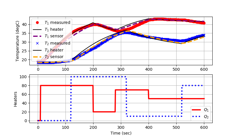
plt.figure() ax=plt.subplot(2,1,1) ax.grid() plt.plot(data['Time'],data['T1'],'ro',label=r'$T_1$ measured') plt.plot(m.time,TH1.value,'k-',label=r'$T_1$ heater') plt.plot(m.time,TC1.value,color='purple',linestyle=, linewidth=3,label=r'$T_1$ sensor') plt.plot(data['Time'],data['T2'],'bx',label=r'$T_2$ measured') plt.plot(m.time,TH2.value,'k-',label=r'$T_2$ heater') plt.plot(m.time,TC2.value,color='orange',linestyle=, linewidth=3,label=r'$T_2$ sensor') plt.ylabel('Temperature (degC)') plt.legend(loc=2) ax=plt.subplot(2,1,2) ax.grid() plt.plot(data['Time'],data['H1'],'r-', linewidth=3,label=r'$Q_1$') plt.plot(data['Time'],data['H2'],'b:', linewidth=3,label=r'$Q_2$') plt.ylabel('Heaters') plt.xlabel('Time (sec)') plt.legend(loc='best') plt.show()

The TCLab is a hands-on application of machine learning and advanced temperature control with two heaters and two temperature sensors. The labs reinforce principles of model development, estimation, and advanced control methods. This is the fifth exercise and it involves estimating parameters in a multi-variate energy balance model with added empirical elements. The predictions are aligned to the measured values through an optimizer that adjusts the parameters to minimize a sum of squared error or sum of absolute values objective. This lab builds upon the TCLab C by using the estimation of parameters in an energy balance but also adding additional equations that give a 2nd order response. The 2nd order response comes from splitting the finite element model of the heaters and temperature sensors. This creates a total of 4 differential equations with parameters that are adjusted to minimize the difference between the predicted and measured temperatures.

Attach:tclab_mhe_hybrid.mp4

  <source src="/do/uploads/Main/tclab_mhe_hybrid.mp4" type="video/mp4">

(:toggle hide gekko_labCm button show="Lab E: Python GEKKO Moving Horizon Estimation":)

(:title TCLab E - Hybrid Model Estimation:) (:keywords Arduino, Hybrid, Parameter, Regression, temperature, control, process control, course:) (:description Regression of Parameters in Multivariate (MIMO) Energy Balance with Empirical Elements using Arduino Data from TCLab:)

The TCLab is a hands-on application of machine learning and advanced temperature control with two heaters and two temperature sensors. The labs reinforce principles of model development, estimation, and advanced control methods. This is the fifth exercise and it involves estimating parameters in a multi-variate energy balance model with added empirical elements. The predictions are aligned to the measured values through an optimizer that adjusts the parameters to minimize a sum of squared error or sum of absolute values objective. This lab builds upon the TCLab C by using the estimation of parameters in an energy balance but also adding additional equations that give a 2nd order response. The 2nd order response comes from splitting the finite element model of the heaters and temperature sensors.

Lab Problem Statement

• Lab E - Hybrid Model Estimation

Data and Solutions

• Solution in Python and MATLAB

(:html:) <iframe width="560" height="315" src="https://www.youtube.com/embed/eEjjkHb1e_E" frameborder="0" allow="accelerometer; autoplay; encrypted-media; gyroscope; picture-in-picture" allowfullscreen></iframe> (:htmlend:)

• Dynamic data, 2 heaters

(:toggle hide gekko_labEd button show="Lab E: Python TCLab Generate Step Data":) (:div id=gekko_labEd:) (:source lang=python:) import numpy as np import pandas as pd import tclab import time import matplotlib.pyplot as plt

1. generate step test data on Arduino

filename = 'tclab_dyn_data2.csv'

1. heater steps

Q1d = np.zeros(601) Q1d[10:200] = 80 Q1d[200:280] = 20 Q1d[280:400] = 70 Q1d[400:] = 50

Q2d = np.zeros(601) Q2d[120:320] = 100 Q2d[320:520] = 10 Q2d[520:] = 80

1. Connect to Arduino

a = tclab.TCLab() fid = open(filename,'w') fid.write('Time,H1,H2,T1,T2\n') fid.close()

1. run step test (10 min)

for i in range(601):

    # set heater values
    a.Q1(Q1d[i])
    a.Q2(Q2d[i])
    print('Time: ' + str(i) +           ' H1: ' + str(Q1d[i]) +           ' H2: ' + str(Q2d[i]) +           ' T1: ' + str(a.T1)   +           ' T2: ' + str(a.T2))
    # wait 1 second
    time.sleep(1)
    fid = open(filename,'a')
    fid.write(str(i)+',str(Q1d[i]),str(Q2d[i]),'               +str(a.T1)+',str(a.T2)\n')

1. close connection to Arduino

a.close()

1. read data file

data = pd.read_csv(filename)

1. plot measurements

plt.figure() plt.subplot(2,1,1) plt.plot(data['Time'],data['H1'],'r-',label='Heater 1') plt.plot(data['Time'],data['H2'],'b--',label='Heater 2') plt.ylabel('Heater (%)') plt.legend(loc='best') plt.subplot(2,1,2) plt.plot(data['Time'],data['T1'],'r.',label='Temperature 1') plt.plot(data['Time'],data['T2'],'b.',label='Temperature 2') plt.ylabel('Temperature (degC)') plt.legend(loc='best') plt.xlabel('Time (sec)') plt.savefig('tclab_dyn_meas2.png')

plt.show() (:sourceend:) (:divend:)

(:toggle hide gekko_labEf button show="Lab E: Python GEKKO Parameter Estimation":) (:div id=gekko_labEf:) (:source lang=python:) (:sourceend:) (:divend:)

(:html:) <video width="550" controls autoplay loop>

  <source src="/do/uploads/Main/tclab_mhe.mp4" type="video/mp4">
  Your browser does not support the video tag.

</video> (:htmlend:)

(:toggle hide gekko_labCm button show="Lab C: Python GEKKO Moving Horizon Estimation":) (:div id=gekko_labCm:) (:source lang=python:) (:sourceend:) (:divend:)

See also:

Advanced Control Lab Overview

GEKKO Documentation

TCLab Documentation

TCLab Files on GitHub

Basic (PID) Control Lab

(:html:) <style> .button {

  border-radius: 4px;
  background-color: #0000ff;
  border: none;
  color: #FFFFFF;
  text-align: center;
  font-size: 28px;
  padding: 20px;
  width: 300px;
  transition: all 0.5s;
  cursor: pointer;
  margin: 5px;

}

.button span {

  cursor: pointer;
  display: inline-block;
  position: relative;
  transition: 0.5s;

}

.button span:after {

  content: '\00bb';
  position: absolute;
  opacity: 0;
  top: 0;
  right: -20px;
  transition: 0.5s;

}

.button:hover span {

  padding-right: 25px;

}

.button:hover span:after {

  opacity: 1;
  right: 0;

} </style> (:htmlend:)