Dynamic Optimization

plt.plot(m.time,p.value,'b-',lw=2)

plt.plot([0,m.time[-1]],[40,40],'k-',lw=3)

    plt.plot(m.time,v[i].value,':',lw=2)

plt.plot(m.time,p.value,'b-',lw=2)

    plt.plot(m.time,v[i].value,':',lw=2)

where v is the controlled variable (CV) with target value of 40.0 and p is the manipulated variable (MV) that can be adjusted between 0 and 100. This is a simple first-order dynamic model that relates the adjustable input p (MV) to the target output v (CV). The rate of change of the MV is limited to 40 every seconds. Determine the stochastic optimal control solution by creating 10 instances of the model that randomly determine the value of K. Optimize this set of models to achieve the target CV value of 40, starting from an initial condition of 0.

where v is the controlled variable (CV) with target range between 38.0 and 40.0, p is the manipulated variable (MV) that can be adjusted between 0 and 100, and `\theta` is the delay. This is a simple first-order dynamic model that relates the adjustable input p (MV) to the target output v (CV). The rate of change of the MV is limited to 40 every seconds. Determine the stochastic optimal control solution by creating 6 instances of the model that randomly determine the delay. Optimize this set of models to achieve the target CV value of between 38 and 40, starting from an initial condition of 0.

Solution 1

Solution 2

where v is the controlled variable (CV) with target value of 40.0 and p is the manipulated variable (MV) that can be adjusted between 0 and 100. This is a simple first-order dynamic model that relates the adjustable input p (MV) to the target output v (CV). The rate of change of the MV is limited to 40 every second. Determine the stochastic optimal control solution by creating 10 instances of the model that randomly determine the value of K. Optimize this set of models to achieve the target CV value of 40, starting from an initial condition of 0.

where v is the controlled variable (CV) with target range between 38.0 and 40.0, p is the manipulated variable (MV) that can be adjusted between 0 and 100, and `\theta` is the delay. This is a simple first-order dynamic model that relates the adjustable input p (MV) to the target output v (CV). The rate of change of the MV is limited to 40 every second. Determine the stochastic optimal control solution by creating 6 instances of the model that randomly determine the delay. Optimize this set of models to achieve the target CV value of between 38 and 40, starting from an initial condition of 0.

$$10 \frac{dv}{dt} = -v + K p$$

$$2 \frac{dv}{dt} = -v + p (t-\theta)$$

Exercise 1

Exercise 2

Consider a system that has an uncertain delay that is uniformly distributed between 1.0 and 5.0. The process model is

`2 \frac{dv}{dt} = -v + p\left(t-\theta\right)`

where v is the controlled variable (CV) with target range between 38.0 and 40.0, p is the manipulated variable (MV) that can be adjusted between 0 and 100. This is a simple first-order dynamic model that relates the adjustable input p (MV) to the target output v (CV). The rate of change of the MV is limited to 40 every second. Determine the stochastic optimal control solution by creating 6 instances of the model that randomly determine the delay. Optimize this set of models to achieve the target CV value of between 38 and 40, starting from an initial condition of 0.

Solution

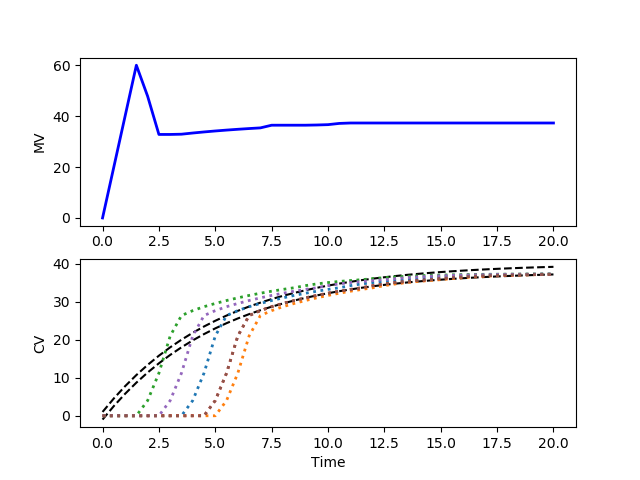
(:toggle hide gekko2 button show="Show Python GEKKO Source":) (:div id=gekko2:) (:source lang=python:) import numpy as np from gekko import GEKKO import matplotlib.pyplot as plt

1. uncertain delay instances

n = 6

m = GEKKO() m.time = np.linspace(0,20,41)

1. manipulated variable

p = m.MV(value=0, lb=0, ub=100) p.STATUS = 1 p.DCOST = 0.1 p.DMAX = 20

1. controlled variable

v = m.Array(m.CV,n) d = m.Array(m.Var,n) for i in range(n):

    delay = np.random.randint(1,11)
    v[i].STATUS = 1
    v[i].SPHI = 40
    v[i].SPLO = 38
    v[i].TAU = 5
    v[i].TR_INIT = 1
    m.delay(p,d[i],delay)
    m.Equation(2*v[i].dt()==-v[i]+d[i])

1. solve optimal control problem

m.options.IMODE = 6 m.options.CV_TYPE = 1 m.solve()

1. get additional solution information

import json with open(m.path+'//results.json') as f:

    results = json.load(f)

1. plot results

plt.figure() plt.subplot(2,1,1) plt.plot(m.time,p.value,'b-',LineWidth=2) plt.ylabel('MV') plt.subplot(2,1,2) plt.plot(m.time,results['v1.tr_hi'],'k--') plt.plot(m.time,results['v1.tr_lo'],'k--') for i in range(n):

    plt.plot(m.time,v[i].value,':',LineWidth=2)

plt.ylabel('CV') plt.xlabel('Time') plt.show() (:sourceend:) (:divend:)

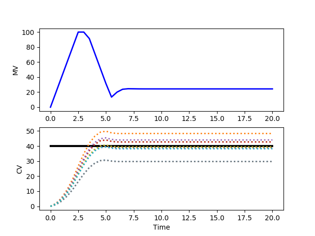
Consider a system that has an uncertain parameter K that is uniformly distributed between 1.0 and 2.0. The process model is

where v is the controlled variable (CV) with target value of 40.0, p is the manipulated variable (MV) that can be adjusted between 0 and 100. This is a simple first-order dynamic model that relates the adjustable input p (MV) to the target output v (CV). The rate of change of the MV is limited to 40 every second. Determine the stochastic optimal control solution by creating 10 instances of the model that randomly determine the value of K. Optimize this set of models to achieve the target CV value of 40, starting from an initial condition of 0.

`10 \frac{dv}{dt} = -v + K p`

(:title Stochastic Optimal Control:) (:keywords multiple objectives, Python, nonlinear control, model predictive control:) (:description Stochastic optimal control is a simultaneous optimization of a distribution of process parameters that are sampled from a set of possible process mathematical descriptions.:)

The underlying model or process parameters that describe a system are rarely known exactly. Optimizing a system with an inaccurate model leads to a sub-optimal solution. If the process model includes uncertain parameters that are described by a distribution function or other set of possible process values, this information can be used directly in the optimal control problem to optimize under uncertainty.

Exercise

Consider a system that has an uncertain parameter K that is uniformly distributed between 10.0 and 11.0. The process model is

`10 \frac{dv}{dt} = -v + K \, p`

where v is the controlled variable (CV) with target value of 40.0, p is the manipulated variable (MV) that can be adjusted between 0 and 100. This is a simple first-order dynamic model that relates the adjustable input p (MV) to the target output v (CV). The rate of change of the MV is limited to 40 every second. Determine the stochastic optimal control solution by creating 10 instances of the model that randomly determine the value of K. Optimize this set of models to achieve the target CV value of 40.

Solution

(:toggle hide gekko button show="Show Python GEKKO Source":) (:div id=gekko:) (:source lang=python:) import numpy as np from gekko import GEKKO import matplotlib.pyplot as plt

1. uncertain parameter

n = 10 K = np.random.rand(n)+1.0

m = GEKKO() m.time = np.linspace(0,20,41)

1. manipulated variable

p = m.MV(value=0, lb=0, ub=100) p.STATUS = 1 p.DCOST = 0.1 p.DMAX = 20

1. controlled variable

v = m.Array(m.CV,n) for i in range(n):

    v[i].STATUS = 1
    v[i].SP = 40
    v[i].TAU = 5
    m.Equation(10*v[i].dt() == -v[i] + K[i]*p)

1. solve optimal control problem

m.options.IMODE = 6 m.options.CV_TYPE = 2 m.solve()

1. plot results

plt.figure() plt.subplot(2,1,1) plt.plot(m.time,p.value,'b-',LineWidth=2) plt.ylabel('MV') plt.subplot(2,1,2) plt.plot([0,m.time[-1]],[40,40],'k-',LineWidth=3) for i in range(n):

    plt.plot(m.time,v[i].value,':',LineWidth=2)

plt.ylabel('CV') plt.xlabel('Time') plt.show() (:sourceend:) (:divend:)