Partial Differential Equations in Python
Main.PartialDifferentialEquations History
Show minor edits - Show changes to markup
$$\rho c_p \frac{\partial T}{\partial t} = -\frac{\partial}{\partial x} \left( k \frac{\partial T}{\partial x} \right) + \dot Q$$
$$\rho c_p \frac{\partial T}{\partial t} = \frac{\partial}{\partial x} \left( k \frac{\partial T}{\partial x} \right) + \dot Q$$
$$\rho c_p \frac{\partial T}{\partial t} = \frac{\partial}{\partial x} \left( k \frac{\partial T}{\partial x} \right) + \dot Q$$
$$\rho c_p \frac{\partial T}{\partial t} = -\frac{\partial}{\partial x} \left( k \frac{\partial T}{\partial x} \right) + \dot Q$$
$$\rho c_p \frac{\partial T}{\partial t} = \frac{\partial}{\partial t} \left( k \frac{\partial T}{\partial t} \right) + \dot Q$$
$$\rho c_p \frac{\partial T}{\partial t} = \frac{\partial}{\partial x} \left( k \frac{\partial T}{\partial x} \right) + \dot Q$$
plt.plot(tm,T1.value,'k-',linewidth=2,label=r'$T_{left}\,(^oC)$')
plt.plot(tm,T1.value,'k-',lw=2,label=r'$T_{left}\,(^oC)$')
plt.plot(tm,T2.value,'b-',linewidth=2,label=r'$T_{right}\,(^oC)$')
plt.plot(tm,T2.value,'b-',lw=2,label=r'$T_{right}\,(^oC)$')
$$\rho c_p \frac{\partial T}{\partial t} = \frac{\partial}{\partial t} \left( k \frac{\partial T}{\partial t} \right) = \dot Q$$
$$\rho c_p \frac{\partial T}{\partial t} = \frac{\partial}{\partial t} \left( k \frac{\partial T}{\partial t} \right) + \dot Q$$
(:html:) <video width="550" controls autoplay loop>
  <source src="/do/uploads/Main/heat_2bvp.mp4" type="video/mp4">
  Your browser does not support the video tag.
</video> (:htmlend:)
- The parabolic PDE equation describes the evolution of temperature
- for the interior region of the rod. This model is modified to make
- one end of the device fixed and the other temperature at the end of the
- device calculated.
import numpy as np from gekko import GEKKO import matplotlib.pyplot as plt import matplotlib.animation as animation
- Steel temperature profile
- Diameter = 3 cm
- Length = 10 cm
seg = 100 # number of segments T_melt = 1426 # melting temperature of H13 steel pi = 3.14159 # pi d = 3 / 100 # diameter (m) L = 10 / 100 # length (m) L_seg = L / seg # length of a segment (m) A = pi * d**2 / 4 # cross-sectional area (m) As = pi * d * L_seg # surface heat transfer area (m^2) heff = 5.8 # heat transfer coeff (W/(m^2*K)) keff = 28.6 # thermal conductivity in H13 steel (W/m-K) rho = 7760 # density of H13 steel (kg/m^3) cp = 460 # heat capacity of H13 steel (J/kg-K) Ts = 23 # temperature of the surroundings (°C)
m = GEKKO() # create GEKKO model
tf = 3000 nt = int(tf/30) + 1 dist = np.linspace(0,L,seg+2) m.time = np.linspace(0,tf,nt) T1 = m.MV(ub=T_melt) # temperature 1 (°C) T1.value = np.ones(nt) * 23 # start at room temperature T1.value[10:] = 80 # step at 300 sec
T = [m.Var(23) for i in range(seg)] # temperature of the segments (°C)
T2 = m.MV(ub=T_melt) # temperature 2 (°C) T2.value = np.ones(nt) * 23 # start at room temperature T2.value[50:] = 100 # step at 300 sec
- Energy balance for the segments
- accumulation =
- (heat gained from upper segment)
- - (heat lost to lower segment)
- - (heat lost to surroundings)
- Units check
- kg/m^3 * m^2 * m * J/kg-K * K/sec =
- W/m-K * m^2 * K / m
- - W/m-K * m^2 * K / m
- - W/m^2-K * m^2 * K
- first segment
m.Equation(rho*A*L_seg*cp*T[0].dt() == keff*A*(T1-T[0])/L_seg - keff*A*(T[0]-T[1])/L_seg - heff*As*(T[0]-Ts))
- middle segments
m.Equations([rho*A*L_seg*cp*T[i].dt() == keff*A*(T[i-1]-T[i])/L_seg - keff*A*(T[i]-T[i+1])/L_seg - heff*As*(T[i]-Ts) for i in range(1,seg-1)])
- last segment
m.Equation(rho*A*L_seg*cp*T[-1].dt() == keff*A*(T[-2]-T[-1])/L_seg - keff*A*(T[-1]-T2)/L_seg - heff*As*(T[-1]-Ts))
- simulation
m.options.IMODE = 4 m.solve()
- plot results
plt.figure() tm = m.time / 60.0 plt.plot(tm,T1.value,'k-',linewidth=2,label=r'$T_{left}\,(^oC)$') plt.plot(tm,T[5].value,':',color='yellow',label=r'$T_{5}\,(^oC)$') plt.plot(tm,T[15].value,,color='red',label=r'$T_{15}\,(^oC)$') plt.plot(tm,T[25].value,,color='green',label=r'$T_{50}\,(^oC)$') plt.plot(tm,T[45].value,'-.',color='gray',label=r'$T_{85}\,(^oC)$') plt.plot(tm,T[95].value,'-',color='orange',label=r'$T_{95}\,(^oC)$') plt.plot(tm,T2.value,'b-',linewidth=2,label=r'$T_{right}\,(^oC)$') plt.ylabel(r'$T\,(^oC$)') plt.xlabel('Time (min)') plt.xlim([0,50]) plt.legend(loc=4) plt.savefig('heat.png')
- create animation as heat.mp4
fig = plt.figure(figsize=(5,4)) fig.set_dpi(300) ax1 = fig.add_subplot(1,1,1)
- store results in d
d = np.empty((seg+2,len(m.time))) d[0] = np.array(T1.value) for i in range(seg):
d[i+1] = np.array(T[i].value)
d[-1] = np.array(T2.value) d = d.T
k = 0 def animate(i):
    global k
    k = min(len(m.time)-1,k)
    ax1.clear()
    plt.plot(dist*100,d[k],color='red',label=r'Temperature ($^oC$)')
    plt.text(1,100,'Elapsed time str(round(m.time[k]/60,2)) min')
    plt.grid(True)
    plt.ylim([20,110])
    plt.xlim([0,L*100])
    plt.ylabel(r'T ($^oC$)')
    plt.xlabel(r'Distance (cm)')
    plt.legend(loc=1)
    k += 1
anim = animation.FuncAnimation(fig,animate,frames=len(m.time),interval=20)
- requires ffmpeg to save mp4 file
- available from https://ffmpeg.zeranoe.com/builds/
- add ffmpeg.exe to path such as C:\ffmpeg\bin\ in
- environment variables
try:
anim.save('heat.mp4',fps=10)
except:
    print('requires ffmpeg to save mp4 file')
    plt.show()
'''Heated Rod (Left Boundary Condition)
Heated Rod (Left Boundary Condition)
'''Heated Rod (Left and Right Boundary Conditions)
Heated Rod (Left and Right Boundary Conditions)
(:toggle hide heat button show="Show GEKKO (Python) Code":)
(:toggle hide heat2 button show="Show GEKKO (Python) Code":)
This code requires ffmpeg to create the animation. If ffmpeg is not available, it does not create the mp4.
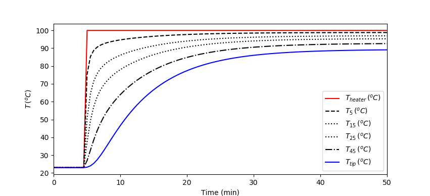
'''Heated Rod (Left Boundary Condition)
The following simulation is for a heated rod (10 cm) with the left side temperature step to 100 oC. The heat transfers to the right by conduction and away from the rod by convection. The temperature at the tip is the lowest temperature because of heat lost by convection to the surrounding air.
(:sourceend:) (:divend:)
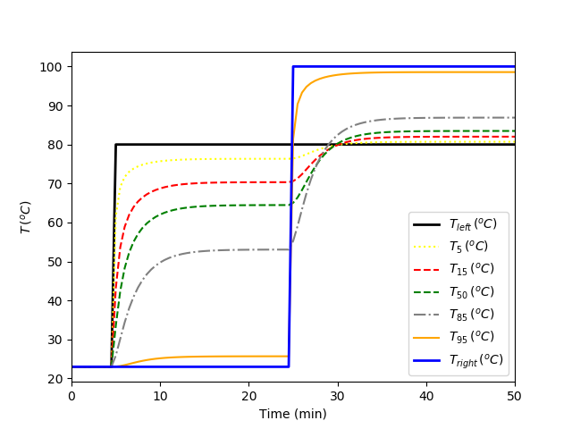
'''Heated Rod (Left and Right Boundary Conditions)
The following simulation is for the same heated rod (10 cm) as above but with the left and right side temperatures specified. The left is stepped up to 80 oC at about 5 minutes and the right is stepped up to 100 oC at about 25 minutes. The heat transfers to the center by conduction and away from the rod by convection.
(:toggle hide heat button show="Show GEKKO (Python) Code":) (:div id=heat2:)
This code requires ffmpeg to create the animation. If ffmpeg is not available, it does not create the mp4.
(:source lang=python:)
- Artificial Lift Rod Pump, See Article
- Artificial Lift Rod Pump (Article, Source Code)
The wave equation solution is described in the GEKKO Paper and work on Artificial Lift Rod Pumping and in the journal publication (Model Predictive Automatic Control of Sucker Rod Pump System with Simulation Case Study (2019).
The wave equation solution is described in the GEKKO Paper and work on Artificial Lift Rod Pumping and in the journal publication Model Predictive Automatic Control of Sucker Rod Pump System with Simulation Case Study (2019).
(:title Partial Differential Equations in Python:) (:keywords dynamic modeling, engineering, differential, algebraic, modeling language, tutorial, partial, PDE:) (:description Solve partial differential equations (PDEs) with Python GEKKO. Examples include the unsteady heat equation and wave equation.:)
When there is spatial and temporal dependence, the transient model is often a partial differntial equation (PDE). Orthogonal Collocation on Finite Elements is reviewed for time discretization. A similar approach can be taken for spatial discretization as well for numerical solution of PDEs. There are analytic (exact and closed form) solutions to PDEs but they are limited to ideal or simplified cases that may not be able to capture the full physics of the problem. For numerical solutions, Finite Element Analysis (FEA) is used to break the simulated object into a grid of discrete points. These discrete points are an approximation of the local quantity of interest. Boundary conditions are specified in space and time and are often the Manipulated Variables for the problem.
Once a PDEs is simulated, it can also be used in estimation or predictive control problems. There are examples of PDE models with Moving Horizon Estimation (MHE) and Model Predictive Control (MPC).
- Artificial Lift Rod Pump, See Article
- Solid Oxide Fuel Cell
Two common PDEs are the heat equation and the wave equation. The wave equation describes the propagation of waves such as in water, sound, and seismic. The heat equation describes the transfer of heat as it flows from high temperature to low temperature regions.
Heat Equation
The heat equation in one dimension is a parabolic PDE. The one dimensional transient heat equation is contains a partial derivative with respect to time and a second partial derivative with respect to distance.
$$\rho c_p \frac{\partial T}{\partial t} = \frac{\partial}{\partial t} \left( k \frac{\partial T}{\partial t} \right) = \dot Q$$
with `\rho` as density, `c_p` as heat capacity, `T` as the temperature, `k` as the thermal conductivity, and `\dot Q` as the heat input rate. The heat equation is discretized in space to give a set of Ordinary Differential Equations (ODEs) in time.
(:toggle hide heat button show="Show GEKKO (Python) Code":) (:div id=heat:) (:source lang=python:)
- The parabolic PDE equation describes the evolution of temperature
- for the interior region of the rod. This model is modified to make
- one end of the rod fixed and the other temperature at the end of the
- rod calculated.
import numpy as np from gekko import GEKKO import matplotlib.pyplot as plt
- Steel rod temperature profile
- Diameter = 3 cm
- Length = 10 cm
seg = 100 # number of segments T_melt = 1426 # melting temperature of H13 steel pi = 3.14159 # pi d = 3 / 100 # rod diameter (m) L = 10 / 100 # rod length (m) L_seg = L / seg # length of a segment (m) A = pi * d**2 / 4 # rod cross-sectional area (m) As = pi * d * L_seg # surface heat transfer area (m^2) heff = 5.8 # heat transfer coeff (W/(m^2*K)) keff = 28.6 # thermal conductivity in H13 steel (W/m-K) rho = 7760 # density of H13 rod steel (kg/m^3) cp = 460 # heat capacity of H13 steel (J/kg-K) Ts = 23 # temperature of the surroundings (°C) c2k = 273.15 # Celcius to Kelvin
m = GEKKO() # create GEKKO model
tf = 3000 nt = int(tf/30) + 1 m.time = np.linspace(0,tf,nt) Th = m.MV(ub=T_melt) # heater temperature (°C) Th.value = np.ones(nt) * 23 # start at room temperature Th.value[10:] = 100 # step at 300 sec
T = [m.Var(23) for i in range(seg)] # temperature of the segments (°C)
- Energy balance for the rod (segments)
- accumulation =
- (heat gained from upper segment)
- - (heat lost to lower segment)
- - (heat lost to surroundings)
- Units check
- kg/m^3 * m^2 * m * J/kg-K * K/sec =
- W/m-K * m^2 * K / m
- - W/m-K * m^2 * K / m
- - W/m^2-K * m^2 * K
- first segment
m.Equation(rho*A*L_seg*cp*T[0].dt() == keff*A*(Th-T[0])/L_seg - keff*A*(T[0]-T[1])/L_seg - heff*As*(T[0]-Ts))
- middle segments
m.Equations([rho*A*L_seg*cp*T[i].dt() == keff*A*(T[i-1]-T[i])/L_seg - keff*A*(T[i]-T[i+1])/L_seg - heff*As*(T[i]-Ts) for i in range(1,seg-1)])
- last segment
m.Equation(rho*A*L_seg*cp*T[seg-1].dt() == keff*A*(T[seg-2]-T[seg-1])/L_seg - heff*(As+A)*(T[seg-1]-Ts))
- simulation
m.options.IMODE = 4 m.solve()
- plot results
plt.figure() tm = m.time / 60.0 plt.plot(tm,Th.value,'r-',label=r'$T_{heater}\,(^oC)$') plt.plot(tm,T[5].value,'k--',label=r'$T_5\,(^oC)$') plt.plot(tm,T[15].value,'k:',label=r'$T_{15}\,(^oC)$') plt.plot(tm,T[25].value,'k:',label=r'$T_{25}\,(^oC)$') plt.plot(tm,T[45].value,'k-.',label=r'$T_{45}\,(^oC)$') plt.plot(tm,T[-1].value,'b-',label=r'$T_{tip}\,(^oC)$') plt.ylabel(r'$T\,(^oC$)') plt.xlabel('Time (min)') plt.xlim([0,50]) plt.legend(loc=4) plt.show() (:sourceend:) (:divend:)
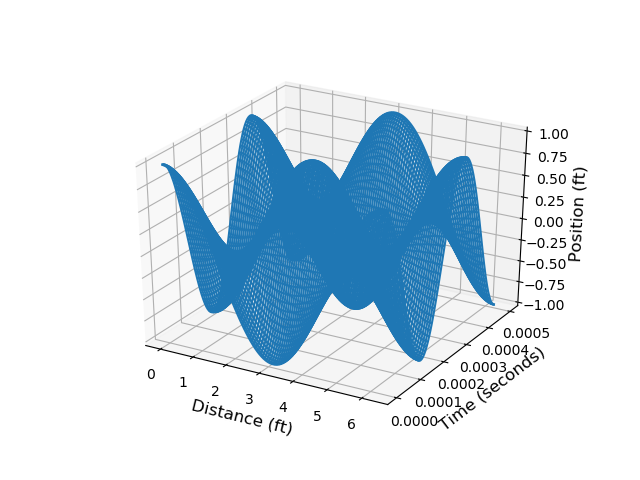
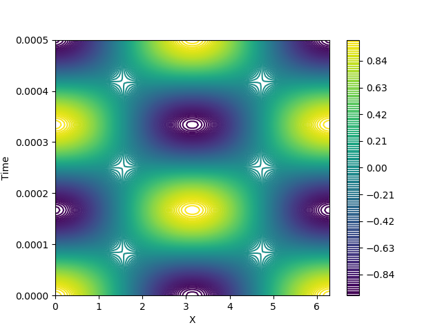
Wave Equation
The wave equation solution is described in the GEKKO Paper and work on Artificial Lift Rod Pumping and in the journal publication (Model Predictive Automatic Control of Sucker Rod Pump System with Simulation Case Study (2019).
(:toggle hide wave button show="Show GEKKO (Python) Code":) (:div id=wave:)
(:source lang=python:) import numpy as np import matplotlib.pyplot as plt from gekko import* from mpl_toolkits.mplot3d.axes3d import Axes3D
tf = .0005 npt = 100 xf = 2*np.pi npx = 100 time = np.linspace(0,tf,npt) xpos = np.linspace(0,xf,npx)
m = GEKKO() m.time = time
def phi(x):
    phi = np.cos(x)
    return phi
def psi(x):
    psi = np.sin(2*x)
    return psi
x0 = phi(xpos) v0 = psi(xpos) dx = xpos[1]-xpos[0] a = 18996.06 c = m.Const(value = a) dx = m.Const(value = dx) u = [m.Var(value = x0[i]) for i in range(npx)] v = [m.Var(value = v0[i]) for i in range(npx)] [m.Equation(u[i].dt()==v[i]) for i in range(npx)] m.Equation(v[0].dt()==c**2 * (u[1] - 2.0*u[0] + u[npx-1])/dx**2 ) [m.Equation(v[i+1].dt()== c**2 * (u[i+2] - 2.0*u[i+1] + u[i])/dx**2) for i in range(npx-2) ] m.Equation(v[npx-1].dt()== c**2 * (u[npx-2] - 2.0*u[npx-1] + u[0])/dx**2 ) m.options.imode = 4 m.options.solver = 1 m.options.nodes = 3
m.solve()
- re-arrange results for plotting
for i in range(npx):
    if i ==0:
        ustor = np.array([u[i]])
        tstor = np.array([m.time])
    else:
        ustor = np.vstack([ustor,u[i]])
        tstor = np.vstack([tstor,m.time])
for i in range(npt):
    if i == 0:
        xstor = xpos
    else:
        xstor = np.vstack([xstor,xpos])
xstor = xstor.T t = tstor ustor = np.array(ustor)
fig = plt.figure() ax = fig.add_subplot(1,1,1,projection='3d') ax.set_xlabel('Distance (ft)', fontsize = 12) ax.set_ylabel('Time (seconds)', fontsize = 12) ax.set_zlabel('Position (ft)', fontsize = 12) ax.set_zlim((-1,1)) p = ax.plot_wireframe(xstor,tstor,ustor, rstride=1,cstride=1) fig.savefig('wave_3d.png', Transparent=True)
plt.figure() plt.contour(xstor, tstor, ustor, 150) plt.colorbar() plt.xlabel('X') plt.ylabel('Time') plt.savefig('wave_contour.png', Transparent=True) plt.show() (:sourceend:) (:divend:)