Dynamic Optimization

(:toggle hide ex1 button show="Automated Collocation with Python Gekko":)

(:toggle hide ex1 button show="Automation Collocation with Python Gekko":) (:div id=ex1:) (:source lang=python:) from gekko import GEKKO m = GEKKO(remote=False) # create GEKKO model y = m.Var(5.0,name='y') # create GEKKO variable m.Equation(y.dt()==-y) # create GEKKO equation m.time = [0,1,2,3] # time points m.options.IMODE = 4 # simulation mode m.options.NODES = 4 # set NODES=4 m.options.CSV_WRITE=2 # write results_all.json

                        #   with internal nodes

m.solve(disp=False) # solve (:sourceend:) (:divend:)

(:toggle hide ex2 button show="Manual Collocation with Python Gekko":) (:div id=ex2:) (:source lang=python:) import numpy as np N = np.array()

time = np.array([0.0, 0.5-np.sqrt(5)/10.0, 0.5+np.sqrt(5)/10.0, 1.0])

from gekko import GEKKO m = GEKKO() y0 = 5 y = m.Array(m.Var,3,value=0) dy = m.Array(m.Var,3,value=0)

Ndy = np.dot(N,dy) m.Equations([Ndy[i]==(y[i]-y0) for i in range(3)]) m.Equations([dy[i]+y[i]==0 for i in range(3)]) m.solve(disp=False) print(y) (:sourceend:) (:divend:)

(:toggle hide ex3 button show="Manual Collocation with Python Scipy":) (:div id=ex3:) (:source lang=python:) import numpy as np N = np.array()

time = np.array([0.0, 0.5-np.sqrt(5)/10.0, 0.5+np.sqrt(5)/10.0, 1.0])

from scipy.optimize import fsolve

y0 = 5 zGuess = np.zeros(6) # y1-y3 and dydt1-dydt3

def myFunction(z):

    y  = z[0:3]
    dy = z[3:6]

    F = np.empty(6)
    F[0:3] = np.dot(N,dy) - (y-y0)
    F[3:7] = dy + y
    return F

z = fsolve(myFunction,zGuess) print(z) (:sourceend:) (:divend:)

(:html:) <iframe width="560" height="315" src="https://www.youtube.com/embed/Avwn53krkgY" frameborder="0" allow="accelerometer; autoplay; clipboard-write; encrypted-media; gyroscope; picture-in-picture" allowfullscreen></iframe> (:htmlend:)

• Solution on Google Colab with Both Notebooks on GitHub

• Solution on Google Colab
• Notebooks on GitHub

• Collocation Activity Solution on Google Colab

• Collocation Activity on Google Colab
• Collocation Activity on Google Colab
• Collocation Activity Notebooks on GitHub

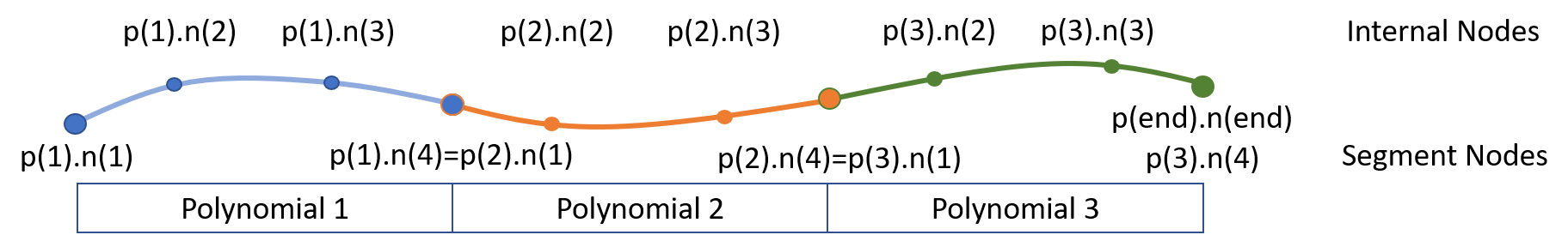
Discretization of a continuous time representation allow large-scale nonlinear programming (NLP) solvers to find solutions at specified intervals in a time horizon.

• Collocation Activity on Google Colab with Collocation Activity on Google Colab or source.

There are many names and related techniques for obtaining mathematical relationships between derivatives and non-derivative values. Some of the terms that are relevant to this discussion include orthogonal collocation on finite elements, direct transcription, Gauss pseudospectral method, Gaussian quadrature, Lobatto quadrature, Radau collocation, Legendre polynomials, Chebyshev polynomials, Jacobi polynomials, Laguerre polynomials, any many more. There are many papers that discuss the details of the derivation and theory behind these methods^1-5. The purpose of this section is to give a practical introduction to orthogonal collocation on finite elements with Lobatto quadrature for the numerical solution of differential algebraic equations. See the documentation on Nodes for additional details on displaying the internal nodes.

Discretization of a continuous time representation allow large-scale nonlinear programming (NLP) solvers to find solutions at specified intervals in a time horizon. There are many names and related techniques for obtaining mathematical relationships between derivatives and non-derivative values. Some of the terms that are relevant to this discussion include orthogonal collocation on finite elements, direct transcription, Gauss pseudospectral method, Gaussian quadrature, Lobatto quadrature, Radau collocation, Legendre polynomials, Chebyshev polynomials, Jacobi polynomials, Laguerre polynomials, any many more. There are many papers that discuss the details of the derivation and theory behind these methods^1-5. The purpose of this section is to give a practical introduction to orthogonal collocation on finite elements with Lobatto quadrature for the numerical solution of differential algebraic equations. See the documentation on Nodes for additional details on displaying the internal nodes.

    plt.plot(tc(n),yc,'o',markersize=10)

from APMonitor.apm import *

(:toggle hide python button show="Show APM Python Source":)

    m = GEKKO()

    u = m.Param(value=4)
    x = m.Var(value=0)
    m.Equation(5*x.dt() == -x**2 + u)

    m.time = [0,tf]

    m.options.imode = 4
    m.options.time_shift = 0

    plt.plot(tc(n),yc,'o',markersize=10,label='Nodes = '+str(i))

plt.legend(loc='best')

    #m.clear()#apm(s,a,'clear all') # clear prior application

(:html:) <iframe width="560" height="315" src="https://www.youtube.com/embed/0UL-Y_mEIuI" frameborder="0" allow="autoplay; encrypted-media" allowfullscreen></iframe> (:htmlend:)

(:toggle hide solution1 button show="Show Solution 1":) (:div id=solution1:)

(:html:) <iframe width="560" height="315" src="https://www.youtube.com/embed/DBjmW4Lwpjc?rel=0" frameborder="0" allowfullscreen></iframe> (:htmlend:) (:divend:)

(:toggle hide solution2 button show="Show Solution 2":) (:div id=solution2:)

(:divend:)

(:toggle hide python button show="APM Python Source":)

(:toggle hide gekko button show="Show GEKKO (Python) Code":) (:div id=gekko:) (:source lang=python:) from __future__ import division import numpy as np from scipy.optimize import fsolve from scipy.integrate import odeint import matplotlib.pyplot as plt

1. final time

tf = 1.0

1. solve with ODEINT (for comparison)

def model(x,t):

    u = 4.0
    return (-x**2 + u)/5.0

t = np.linspace(0,tf,20) y0 = 0 y = odeint(model,y0,t) plt.figure(1) plt.plot(t,y,'r-',label='ODEINT')

1. ----------------------------------------------------
2. Approach #1 - Write the model equations in Python
3. ----------------------------------------------------
4. define collocation matrices

def colloc(n):

    if (n==2):
        NC = np.array(1.0?)
    if (n==3):
        NC = np.array()
    if (n==4):
        NC = np.array()
    if (n==5):
        NC = np.array()
    if (n==6):
        NC = np.array([[0.191, -0.147, 0.139, -0.113, 0.047],
                       [0.276,  0.059, 0.051, -0.050, 0.022],
                       [0.267,  0.193, 0.252, -0.114, 0.045],
                       [0.269,  0.178, 0.384,  0.032, 0.019],
                       [0.269,  0.181, 0.374,  0.110, 0.067]])
    return NC

1. define collocation points from Lobatto quadrature

def tc(n):

    if (n==2):
        time = np.array([0.0,1.0])
    if (n==3):
        time = np.array([0.0,0.5,1.0])
    if (n==4):
        time = np.array([0.0,                          0.5-np.sqrt(5)/10.0,                          0.5+np.sqrt(5)/10.0,                          1.0])
    if (n==5):
        time = np.array([0.0,0.5-np.sqrt(21)/14.0,                          0.5,0.5+np.sqrt(21)/14.0, 1])
    if (n==6):
        time = np.array([0.0,                          0.5-np.sqrt((7.0+2.0*np.sqrt(7.0))/21.0)/2.0,                          0.5-np.sqrt((7.0-2.0*np.sqrt(7.0))/21.0)/2.0,                          0.5+np.sqrt((7.0-2.0*np.sqrt(7.0))/21.0)/2.0,                          0.5+np.sqrt((7.0+2.0*np.sqrt(7.0))/21.0)/2.0,                          1.0])
    return time*tf

1. solve with SciPy fsolve

def myFunction(z,*param):

    n = param[0]
    m = param[1]
    # rename z as x and xdot variables
    x = np.empty(n-1)
    xdot = np.empty(n-1)
    x[0:n-1] = z[0:n-1]
    xdot[0:n-1] = z[n-1:m]

    # initial condition (x0)
    x0 = 0.0
    # input parameter (u)
    u = 4.0
    # final time
    tn = tf

    # function evaluation residuals
    F = np.empty(m)
    # nonlinear differential equations at each node
    # 5 dx/dt = -x^2 + u
    F[0:n-1] = 5.0 * xdot[0:n-1] + x[0:n-1]**2 - u
    # collocation equations
    # tn * NC * xdot = x - x0
    NC = colloc(n)
    F[n-1:m] = tn * np.dot(NC,xdot) - x + x0 * np.ones(n-1)
    return F

sol_py = np.empty(5) # store 5 results for i in range(2,7):

    n = i
    m = (i-1)*2
    zGuess = np.ones(m)
    z = fsolve(myFunction,zGuess,args=(n,m))
    # add to plot
    yc = np.insert(z[0:n-1],0,0)
    plt.plot(tc(n),yc,'o',markersize=20)
    # store just the last x[n] value
    sol_py[i-2] = z[n-2]

1. ----------------------------------------------------
2. Approach #2 - Write model in APMonitor and let
3. modeling language create the collocation equations
4. ----------------------------------------------------
5. load GEKKO

from gekko import GEKKO

m = GEKKO()

u = m.Param(value=4) x = m.Var(value=0) m.Equation(5*x.dt() == -x**2 + u)

m.time = [0,tf]

m.options.imode = 4

sol_apm = np.empty(5) # store 5 results i = 0 for nodes in range(2,7):

    m.clear()#apm(s,a,'clear all') # clear prior application
    m.options.nodes = nodes
    m.solve() # solve problem
    sol_apm[i] = x.value[-1] # store solution (last point)
    i += 1

1. print the solutions

print(sol_py) print(sol_apm)

1. show plot

plt.ylabel('x(t)') plt.xlabel('time') plt.show() (:sourceend:) (:divend:)

(:toggle hide python button show="Python Source":)

(:html:) <iframe width="560" height="315" src="https://www.youtube.com/embed/DBjmW4Lwpjc?rel=0" frameborder="0" allowfullscreen></iframe> (:htmlend:)

Collocation in MATLAB and Python (APM Solution)

(:html:) <iframe width="560" height="315" src="https://www.youtube.com/embed/DBjmW4Lwpjc?rel=0" frameborder="0" allowfullscreen></iframe> (:htmlend:)

(:toggle hide python button show="Buy or Build TCLab":) (:div id=python:)

(:divend:)

Objective: Solve a differential equation with orthogonal collocation on finite elements. Create a MATLAB or Python script to simulate and display the results. Estimated Time: 2-3 hours

(:source lang=python:) import numpy as np from scipy.optimize import fsolve from scipy.integrate import odeint import matplotlib.pyplot as plt

1. final time

tf = 1.0

1. solve with ODEINT (for comparison)

def model(x,t):

    u = 4.0
    return (-x**2 + u)/5.0

t = np.linspace(0,tf,20) y0 = 0 y = odeint(model,y0,t) plt.figure(1) plt.plot(t,y,'r-',label='ODEINT')

1. ----------------------------------------------------
2. Approach #1 - Write the model equations in Python
3. ----------------------------------------------------
4. define collocation matrices

def colloc(n):

    if (n==2):
        NC = np.array(1.0?)
    if (n==3):
        NC = np.array()
    if (n==4):
        NC = np.array()
    if (n==5):
        NC = np.array()
    if (n==6):
        NC = np.array([[0.191, -0.147, 0.139, -0.113, 0.047],
                       [0.276,  0.059, 0.051, -0.050, 0.022],
                       [0.267,  0.193, 0.252, -0.114, 0.045],
                       [0.269,  0.178, 0.384,  0.032, 0.019],
                       [0.269,  0.181, 0.374,  0.110, 0.067]])
    return NC

1. define collocation points from Lobatto quadrature

def tc(n):

    if (n==2):
        time = np.array([0.0,1.0])
    if (n==3):
        time = np.array([0.0,0.5,1.0])
    if (n==4):
        time = np.array([0.0,                          0.5-np.sqrt(5)/10.0,                          0.5+np.sqrt(5)/10.0,                          1.0])
    if (n==5):
        time = np.array([0.0,0.5-np.sqrt(21)/14.0,                          0.5,0.5+np.sqrt(21)/14.0, 1])
    if (n==6):
        time = np.array([0.0,                          0.5-np.sqrt((7.0+2.0*np.sqrt(7.0))/21.0)/2.0,                          0.5-np.sqrt((7.0-2.0*np.sqrt(7.0))/21.0)/2.0,                          0.5+np.sqrt((7.0-2.0*np.sqrt(7.0))/21.0)/2.0,                          0.5+np.sqrt((7.0+2.0*np.sqrt(7.0))/21.0)/2.0,                          1.0])
    return time*tf

1. solve with SciPy fsolve

def myFunction(z,*param):

    n = param[0]
    m = param[1]
    # rename z as x and xdot variables
    x = np.empty(n-1)
    xdot = np.empty(n-1)
    x[0:n-1] = z[0:n-1]
    xdot[0:n-1] = z[n-1:m]

    # initial condition (x0)
    x0 = 0.0
    # input parameter (u)
    u = 4.0
    # final time
    tn = tf

    # function evaluation residuals
    F = np.empty(m)
    # nonlinear differential equations at each node
    # 5 dx/dt = -x^2 + u
    F[0:n-1] = 5.0 * xdot[0:n-1] + x[0:n-1]**2 - u
    # collocation equations
    # tn * NC * xdot = x - x0
    NC = colloc(n)
    F[n-1:m] = tn * np.dot(NC,xdot) - x + x0 * np.ones(n-1)
    return F

sol_py = np.empty(5) # store 5 results for i in range(2,7):

    n = i
    m = (i-1)*2
    zGuess = np.ones(m)
    z = fsolve(myFunction,zGuess,args=(n,m))
    # add to plot
    yc = np.insert(z[0:n-1],0,0)
    plt.plot(tc(n),yc,'o',markersize=20)
    # store just the last x[n] value
    sol_py[i-2] = z[n-2]

1. ----------------------------------------------------
2. Approach #2 - Write model in APMonitor and let
3. modeling language create the collocation equations
4. ----------------------------------------------------
5. load APM package

try:

    from APMonitor import *

except:

    # Automatically install APMonitor
    import pip
    pip.main(['install','APMonitor'])
    try:
        from APMonitor import *
    except:
        print('pip installation unsuccessful')
        print('Visit apmonitor.com to download apm.py')
        from apm import *

s = 'https://byu.apmonitor.com' a = 'node_test'

fid = open('collocation.apm','w')

1. write model

fid.write('Parameters \n') fid.write(' u = 4 \n') fid.write('Variables \n') fid.write(' x = 0 \n') fid.write('Equations \n') fid.write(' 5 * $x = -x^2 + u \n')

1. close file

fid.close()

fid = open('collocation.csv','w')

1. write data file

fid.write('time \n') fid.write('0 \n') fid.write(str(tf)+'\n')

1. close file

fid.close()

sol_apm = np.empty(5) # store 5 results i = 0 for nodes in range(2,7):

    apm(s,a,'clear all') # clear prior application
    apm_load(s,a,'collocation.apm') # load model
    csv_load(s,a,'collocation.csv') # load data
    apm_option(s,a,'nlc.imode',4)   # imode = 4, simulation
    apm_option(s,a,'nlc.nodes',nodes) # nodes (2-6)
    apm(s,a,'solve') # solve problem
    y = apm_sol(s,a) # retrieve solution
    sol_apm[i] = y['x'][-1] # store solution (last point)
    i += 1

1. print the solutions

print(sol_py) print(sol_apm)

1. show plot

plt.ylabel('x(t)') plt.xlabel('time') plt.show() (:sourceend:)

Compare orthogonal collocation on finite elements with 3 nodes with a numerical integrator (e.g. ODE15s in MATLAB or ODEINT in Python). Calculate the error at each of the solution points for the equation (same as for Exercise 1):

 5 dx/dt = -x2 + u

(:html:) <iframe width="560" height="315" src="https://www.youtube.com/embed/8LmIqeuHGL0" frameborder="0" allowfullscreen></iframe> (:htmlend:)

Exercise 1

Solution 1

Collocation in MATLAB and Python (APM Solution)

Exercise 2

Compare orthogonal collocation on finite elements with 3 nodes with a numerical integrator (e.g. ODE15s in MATLAB or ODEINT in Python). Calculate the error at each of the solution points.

Solution 2

Collocation Solution (APM, ODE15s (MATLAB), ODEINT (Python) Compared)

1. Kameswaran, S., Biegler, L.T., Convergence rates for direct transcription of optimal control problems using collocation at Radau points, Computational Optimization and Applications, 41 (1), pp. 81-126, 2008, DOI: 10.1007/s10589-007-9098-9.

Discretization of a continuous time representation allow large-scale nonlinear programming (NLP) solvers to find solutions at specified intervals in a time horizon. There are many names and related techniques for obtaining mathematical relationships between derivatives and non-derivative values. Some of the terms that are relevant to this discussion include orthogonal collocation on finite elements, direct transcription, Gauss pseudospectral method, Gaussian quadrature, Lobatto quadrature, Radau collocation, Legendre polynomials, Chebyshev polynomials, Jacobi polynomials, Laguerre polynomials, any many more. There are many papers that discuss the details of the derivation and theory behind these methods^1-5. The purpose of this section is to give a practical introduction to orthogonal collocation on finite elements with Lobatto quadrature for the numerical solution of differential algebraic equations.

<iframe width="560" height="315" src="https://www.youtube.com/embed/DBjmW4Lwpjc?rel=0" frameborder="0" allowfullscreen></iframe>

(:htmlend:)

Exercise

Objective: Solve a differential equation with orthogonal collocation on finite elements. Create a MATLAB or Python script to simulate and display the results. Estimated Time: 1 hour

Solve the following differential equation from time 0 to 1 with orthogonal collocation on finite elements with 4 nodes for discretization in time.

 5 dx/dt = -x2 + u

Specify the initial condition for x as 0 and the value of the input, u, as 4. Compare the solution result with 2-6 time points (nodes). Report the solution at the final time for each and comment on how the solution changes with an increase in the number of nodes.

Solution

Collocation Exercise in MATLAB

(:html:) <iframe width="560" height="315" src="https://www.youtube.com/embed/0Et07u336Bo?rel=0" frameborder="0" allowfullscreen></iframe>

There are many papers that discuss the details of the derivation and theory behind these methods^1-5. The purpose of this section is to give a practical introduction to orthogonal collocation on finite elements with Lobatto quadrature for the numerical solution of differential algebraic equations.

1. Hedengren, J. D. and Asgharzadeh Shishavan, R., Powell, K.M., and Edgar, T.F., Nonlinear Modeling, Estimation and Predictive Control in APMonitor, Computers & Chemical Engineering, Volume 70, pg. 133–148, 2014. Available at: ScienceDirect or ResearchGate
2. Cizniar, M., Salhi, D., Fikar, M., and Latifi, M.A., A Matlab Package for Orthogonal Collocations on Finite Elements in Dynamic Optimization, 15th Int. Conference Process Control, June 7-10, 2015. Article
3. Renfro, J., Morshedi, A., Asbjornsen, O., Simultaneous Optimization and Solution of Systems Described by Differential/Algebraic Equations, Computers & Chemical Engineering, Volume 11, Number 5, pp. 503-517, 1987.
4. Finlayson, B., Orthogonal Collocation on Finite Elements for PDE Discretization and Solution
5. Biegler, L.T., Solution of Dynamic Optimization Problems by Successive Quadratic Programming and Orthogonal Collocation, Computers & Chemical Engineering, Volume 8, Number 3/4, pp. 243-248, 1984.

1. Nonlinear Modeling, Estimation and Predictive Control in APMonitor, Hedengren, J. D. and Asgharzadeh Shishavan, R., Powell, K.M., and Edgar, T.F., Computers and Chemical Engineering, Volume 70, pg. 133–148, 2014. Available at: ScienceDirect or ResearchGate

<iframe width="560" height="315" src="https://www.youtube.com/embed/sxFTAF_xtLg?rel=0" frameborder="0" allowfullscreen></iframe>

<iframe width="560" height="315" src="https://www.youtube.com/embed/WCTTY4baYLk?rel=0" frameborder="0" allowfullscreen></iframe>

There are many papers that discuss the details of the derivation and theory behind these methods¹. The purpose of this section is to give a practical introduction to orthogonal collocation on finite elements with Lobatto quadrature for the numerical solution of differential algebraic equations.

There are many papers that discuss the details of the derivation and theory behind these methods¹. The purpose of this section is to give a practical introduction to orthogonal collocation on finite elements for the numerical solution of differential algebraic equations.

References

1. Nonlinear Modeling, Estimation and Predictive Control in APMonitor, Hedengren, J. D. and Asgharzadeh Shishavan, R., Powell, K.M., and Edgar, T.F., Computers and Chemical Engineering, Volume 70, pg. 133–148, 2014. Available at: https://dx.doi.org/10.1016/j.compchemeng.2014.04.013

(:title Orthogonal Collocation on Finite Elements:) (:keywords direct transcription, orthogonal collocation, modeling language, differential, algebraic, tutorial:) (:description Collocation methods are used to convert a differential algebraic model into a nonlinear programming problem that can be solved with NLP solvers:)

Discretization of a continuous time representation allow large-scale nonlinear programming (NLP) solvers to find solutions at specified intervals in a time horizon. There are many names and related techniques for obtaining mathematical relationships between derivatives and non-derivative values. Some of the terms that are relevant to this discussion include:

• Orthogonal collocation on finite elements
• Direct transcription
• Gauss pseudospectral method
• Gaussian quadrature
• Lobatto quadrature
• Radau collocation
• Legendre polynomials
• Chebyshev polynomials
• Jacobi polynomials
• Laguerre polynomials
• Any many more...

There are many excellent papers that discuss the details of the derivation and theory behind these methods. The purpose of this section is to give a practical introduction to orthogonal collocation on finite elements for the numerical solution of differential algebraic equations.

Orthogonal Collocation in MATLAB

(:html:) <iframe width="560" height="315" src="https://www.youtube.com/embed/2FeOaGUQwKA?rel=0" frameborder="0" allowfullscreen></iframe> (:htmlend:)