Dynamic Optimization

plt.plot(solution1['time'],solution1['p'],'k-',lw=2) plt.plot(solution2['time'],solution2['p'],'b--',lw=2)

plt.plot(solution1['time'],solution1['x'],'r--',lw=2) plt.plot(solution2['time'],solution2['x'],'g:',lw=2)

The spread of HIV in a patient is approximated with balance equations on (H)ealthy, (I)nfected, and (V)irus population counts². Additional information on the HIV model is at the Process Dynamic and Control Course.

(:toggle hide init1 button show="Show APM Python Code":) (:div id=init1:)

from APMonitor.apm import * # pip install APMonitor

(:divend:)

(:toggle hide init2 button show="Show APM Python Code":) (:div id=init2:)

from APMonitor.apm import * # pip install APMonitor

(:divend:)

(:toggle hide gekko_hiv button show="Show GEKKO (Python) Code":) (:div id=gekko_hiv:) (:source lang=python:) from gekko import GEKKO import numpy as np

1. Manually enter guesses for parameters

lkr = [3,np.log10(0.1),np.log10(2e-7), np.log10(0.5),np.log10(5),np.log10(100)]

1. Model

m = GEKKO()

1. Time

m.time = np.linspace(0,15,61)

1. Parameters to estimate

lg10_kr = [m.FV(value=lkr[i]) for i in range(6)]

1. Variables

kr = [m.Var() for i in range(6)] H = m.Var(value=1e6) I = m.Var(value=0) V = m.Var(value=1e2)

1. Variable to match with data

LV = m.CV(value=2)

1. Equations

m.Equations([10**lg10_kr[i]==kr[i] for i in range(6)]) m.Equations([H.dt() == kr[0] - kr[1]*H - kr[2]*H*V,

             I.dt() == kr[2]*H*V - kr[3]*I,
             V.dt() == -kr[2]*H*V - kr[4]*V + kr[5]*I, 
             LV == m.log10(V)])

1. option #1 for initialization
2. m.options.IMODE = 7 # sequential simulation
3. option #2 for initialization

m.options.IMODE = 4 #simultaneous simulation m.options.COLDSTART = 2

m.options.SOLVER = 1 m.options.MAX_ITER = 1000

m.solve(disp=False)

1. patient virus count data

data = np.array()

1. Convert log-scaled data for plotting

log_v = data[:,1] # 2nd column of data v = np.power(10,log_v)

1. Plot results

import matplotlib.pyplot as plt plt.figure(1) plt.semilogy(m.time,H,'b-') plt.semilogy(m.time,I,'g:') plt.semilogy(m.time,V,'r--') plt.semilogy(data[:,][:,0],v,'ro') plt.xlabel('Time (yr)') plt.ylabel('States (log scale)') plt.legend(['H','I','V']) plt.show() (:sourceend:) (:divend:)

fid.write(' m =str(m) \n')

fid.write(' p[1:n][1::m] \n')

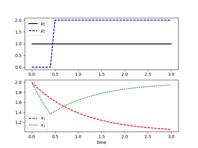
The following example is a demonstration of inserting different initial conditions or parameter values at points throughout the time horizon. A simulation solution is used to provide guess values for a subsequent simulation. The parameter CSV_READ can be set to 2 to provide the initial values for a calculated state. The default (CSV_READ=1) only updates the fixed values and skips the values that are calculated by the solver. Setting COLDSTART >= 1 also has the effect of using calculated values in the CSV file as initial guesses for the solver.

Simulation is a first step after the model development to verify convergence, validate the model response to input changes, and manually adjust parameters to fit an expected response. This section demonstrates how to set up and initialize a dynamic model simulation. Options such as CSV_READ control how much information is read from a data (CSV) file.

The following example is a demonstration of inserting different initial conditions or parameter values at points throughout the time horizon. A simulation solution is used to provide guess values for a subsequent simulation. The parameter CSV_READ can be set to 2 to provide the initial values for a calculated state. The default (CSV_READ=1) only updates the fixed values and skips the values that are calculated by the solver.

Simulation is a first step after the model development to verify convergence, validate the model response to input changes, and manually adjust parameters to fit an expected response. This section demonstrates how to set up and initialize a dynamic model simulation. Options such as CSV_READ? control how much information is read from a data (CSV) file.

A first example shows how to use a scripting language such as MATLAB or Python to provide input values for a matrix of parameters.

The following example is a demonstration of inserting different initial conditions or parameter values at points throughout the time horizon. A simulation solution is used to provide guess values for a subsequent simulation. The parameter CSV_READ? can be set to 2 to provide the initial values for a calculated state. The default (CSV_READ=1) only updates the fixed values and skips the values that are calculated by the solver.

(:source lang=python:) from apm import * import numpy as np

A = np.random.random((3,4)) n = np.size(A,0) # rows m = np.size(A,1) # columns

1. write model.apm

fid = open('model.apm','w') fid.write('Constants \n') fid.write(' n =str(n) \n') fid.write(' \n') fid.write('Parameters \n') fid.write(' p[1:str(n)][1::str(m)] \n') fid.write(' \n') fid.write('Variables \n') fid.write(' x \n') fid.write('Equations \n') fid.write(' x=p[1][1] \n') fid.close()

1. write data.csv

fid = open('data.csv','w') for i in range(n):

    for j in range(m):
        fid.write(' p[str(i+1)][str(j+1)], str(A[i,j]) \n')

fid.close()

1. load model, data file, and solve

s = 'https://byu.apmonitor.com' a = 'matrix_write' apm(s,a,'clear all') apm_load(s,a,'model.apm') csv_load(s,a,'data.csv') apm(s,a,'solve')

1. retrieve solution

apm_web_var(s,a) (:sourceend:)

(:source lang=python:) import numpy as np from apm import * # load APMonitor library

1. Step #1 - Solve model with p = 1
2. Step #1a - write data.csv

n = 31 time = np.linspace(0,3,n) p = np.ones(31) x = 2 * np.ones(31)

fid = open('data.csv','w')

1. write time row

fid.write('time, ') for i in range(n-1):

    fid.write(str(time[i]) +  ', ')

fid.write(str(time[n-1]) + '\n')

1. write 'p' row (input parameter)

fid.write('p, ') for i in range(n-1):

    fid.write(str(p[i]) +  ', ')

fid.write(str(p[n-1]) + '\n')

1. write 'x' row (state variable initialization)

fid.write('x, ')

1. imode: https://apmonitor.com/wiki/index.php/Main/Modes
2. for imode=4-6, include all initialization values
3. for imode=7-9, include only the initial condition for variables

imode = 7 if ((imode>=4) and (imode<=6)):

    for i in range(n-1):
        fid.write(str(x[i]) + ', ')
    fid.write(str(x[n-1]) + '\n')

else:

    fid.write(str(x[0]) + ', ')
    for i in range(1,n-1):
        fid.write('-, ')
    fid.write('-\n')

1. close file

fid.close()

1. Step 1b - Load and solve model

s = 'https://byu.apmonitor.com' a = 'model_init'

apm(s,a,'clear all') apm_load(s,a,'model.apm') csv_load(s,a,'data.csv')

apm_option(s,a,'apm.time_shift',1) apm_option(s,a,'apm.imode',imode) output1 = apm(s,a,'solve')

1. Step 1c - Retrieve results with solution.csv

solution1 = apm_sol(s,a)

1. Step 2 - Solve again with prior solution for initialization and
2. p as a step from 0 to 2
3. Change to imode = 4 and change p trajectory

p[0:5] = 0.0 p[5:n] = 2.0

1. Step 2a - Write new row at the end of solution.csv

fname = 'solution_' + a + '.csv' fid = open(fname,'a') # append to file fid.write('p, ') for i in range(n-1):

    fid.write(str(p[i]) +  ', ')

fid.write(str(p[n-1]) + '\n')

1. close file

fid.close()

1. Step 2b - Reload csv file for initialization

apm(s,a,'clear csv') csv_load(s,a,fname)

1. Step 2c - Solve again but with new inputs

imode = 4 apm_option(s,a,'apm.time_shift',0) apm_option(s,a,'apm.imode',imode) output2 = apm(s,a,'solve') print(output2)

1. Step 2d - Retrieve results with solution.csv

solution2 = apm_sol(s,a)

1. Step 3 - Create plots

import matplotlib.pyplot as plt

plt.figure(1) plt.subplot(2,1,1) plt.plot(solution1['time'],solution1['p'],'k-',linewidth=2) plt.plot(solution2['time'],solution2['p'],'b--',linewidth=2) plt.legend([r'$p_1$',r'$p_2$']) plt.subplot(2,1,2) plt.plot(solution1['time'],solution1['x'],'r--',linewidth=2) plt.plot(solution2['time'],solution2['x'],'g:',linewidth=2) plt.legend([r'$x_1$',r'$x_2$']) plt.xlabel('time') plt.show() (:sourceend:)

Simulation is a first step after the model development to verify convergence, validate the model response to input changes, and manually adjust parameters to fit an expected response. This section demonstrates how to set up and initialize a dynamic model simulation. A first example shows how to use a scripting language such as MATLAB or Python to provide input values for parameters.

Initialize Parameter Matrix

Although a problem may be written correctly, sometimes the solver fails to find a solution or requires excessive time to find a solution. Initialization strategies are critical in these situations to find a nearby solution that seeds the optimization problem with a starting point that allows convergence¹.

The following example is a demonstration of inserting different initial conditions or parameter values at points throughout the time horizon. A simulation solution is used to provide guess values for a subsequent simulation.

Initialize for Dynamic Simulation

1. Safdarnejad, S.M., Hedengren, J.D., Lewis, N.R., Haseltine, E., Initialization Strategies for Optimization of Dynamic Systems, Computers and Chemical Engineering, 2015, Vol. 78, pp. 39-50, DOI: 10.1016/j.compchemeng.2015.04.016. Article

1. 5.Safdarnejad, S.M., Hedengren, J.D., Lewis, N.R., Haseltine, E., Initialization Strategies for Optimization of Dynamic Systems, Computers and Chemical Engineering, 2015, Vol. 78, pp. 39-50, DOI: 10.1016/j.compchemeng.2015.04.016. Article

1. Lewis, N.R., Hedengren, J.D., Haseltine, E.L., Hybrid Dynamic Optimization Methods for Systems Biology with Efficient Sensitivities, Special Issue on Algorithms and Applications in Dynamic Optimization, Processes, 2015, 3(3), 701-729; doi:10.3390/pr3030701. Article

With guess values for parameters (kr_1..6), approximately match the laboratory data for this patient. A subsequent section introduces methods for parameter estimation by minimizing an objective function.

 dH/dt = kr1 - kr2 H - kr3 H V
 dI/dt = kr3 H V - kr4 I
 dV/dt = -kr3 H V - kr5 V + kr6 I
 LV = log10(V)

 kr1 = new healthy cells
 kr2 = death rate of healthy cells
 kr3 = healthy cells converting to infected cells
 kr4 = death rate of infected cells
 kr5 = death rate of virus
 kr6 = production of virus by infected cells

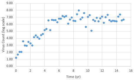
The spread of HIV in a patient is approximated with balance equations on (H)ealthy, (I)nfected, and (V)irus population counts².

 Initial Conditions
 H = healthy cells = 1,000,000
 I = infected cells = 0
 V = virus = 100
 LV = log virus = 2

 Equations
 dH/dt = kr^_1_^ - kr^_2_^ H - kr^_3_^ H V
 dI/dt = kr^_3_^ H V - kr^_4_^ I
 dV/dt = -kr^_3_^ H V - kr^_5_^ V + kr^_6_^ I
 LV = log^_10_^(V)

There are six parameters (kr_1..6) in the model that provide the rates of cell death, infection spread, virus replication, and other processes that determine the spread of HIV in the body.

 Parameters
 kr^_1_^ = new healthy cells
 kr^_2_^ = death rate of healthy cells
 kr^_3_^ = healthy cells converting to infected cells
 kr^_4_^ = death rate of infected cells
 kr^_5_^ = death rate of virus
 kr^_6_^ = production of virus by infected cells

The following data is provided from a virus count over the course of 15 years. Note that the virus count information is reported in log scale.

(:html:) <iframe width="560" height="315" src="https://www.youtube.com/embed/0Et07u336Bo?rel=0" frameborder="0" allowfullscreen></iframe> (:htmlend:)

Although a problem may be written correctly, sometimes the solver fails to find a solution or requires excessive time to find a solution. Initialization strategies are critical in these situations to find a nearby solution that seeds the optimization problem with a starting point that allows convergence¹.

Objective: Simulate a highly nonlinear system, using initialization strategies to find a suitable approximation for a future parameter estimation exercise. Create a MATLAB or Python script to simulate and display the results. Estimated Time: 2 hours

The spread of HIV in a patient is approximated with balance equations on (H)ealthy, (I)nfected, and (V)irus population counts². There are six parameters (kr_1..6) in the model that provide the rates of cell death, infection spread, virus replication, and other processes that determine the spread of HIV in the body. The following data is provided from a virus count over the course of 15 years. Note that the virus count information is reported in log scale.

With guess values for parameters (kr_1..6), approximately match the laboratory data for this patient. A subsequent section introduces methods for parameter estimation by minimizing an objective function.

HIV Simulation in MATLAB and Python

References

1. Safdarnejad, S.M., Hedengren, J.D., Lewis, N.R., Haseltine, E., Initialization Strategies for Optimization of Dynamic Systems, Computers and Chemical Engineering, DOI: 10.1016/j.compchemeng.2015.04.016. Article
2. Nowak, M. and May, R. M. Virus dynamics: mathematical principles of immunology and virology: mathematical principles of immunology and virology. Oxford university press, 2000.

Simulation is a first step in after the model development to verify convergence, validate the model response to input changes, and manually adjust parameters to fit an expected response. This section demonstrates how to set up and solve a dynamic model.

Although a problem may be written correctly, sometimes the solver fails to find a solution or requires excessive time to find a solution. Initialization strategies are critical in these situations to find a nearby solution that seeds the optimization problem with a starting point that allows convergence.

• Safdarnejad, S.M., Hedengren, J.D., Lewis, N.R., Haseltine, E., Initialization Strategies for Optimization of Dynamic Systems, Computers and Chemical Engineering, DOI: 10.1016/j.compchemeng.2015.04.016. Article

Solution

(:htmlend:)

(:title Model Initialization Strategies:)

Simulation is a first step in after the model development to verify convergence, validate the model response to input changes, and manually adjust parameters to fit an expected response. This section demonstrates how to set up and solve a simple dynamic model.

(:html:) <iframe width="560" height="315" src="https://www.youtube.com/embed/-IDTagajoyA" frameborder="0" allowfullscreen></iframe> (:htmlend:)

(:html:) <iframe width="560" height="315" src="https://www.youtube.com/embed/-3FaZEfu7vE" frameborder="0" allowfullscreen></iframe> (:html:)

Exercise

Solution

(:title Initialization Strategies:)

(:title Initialization Strategies for Dynamic Systems:) (:keywords initialization, strategy, modeling language, differential, algebraic, tutorial:) (:description Model initialization strategies for Differential Algebraic Equations (DAEs) with use in dynamic simulation, estimation, and control:)