Practice Midterm Exam 2
Main.MidtermExam2016 History
Show minor edits - Show changes to markup

(:title Midterm Exam for Dynamic Optimization:)
(:title Practice Midterm Exam 2:)
Midterm Exam 2

linewidth=0.5, label=r'$Cases_{db-hi}$')
lw=0.5, label=r'$Cases_{db-hi}$')
linewidth=0.5, label=r'$Cases_{db-lo}$')
lw=0.5, label=r'$Cases_{db-lo}$')
plt.plot(m.time,cases_SPHI, 'k-.', linewidth=0.5,\
plt.plot(m.time,cases_SPHI, 'k-.', lw=0.5,\
plt.plot(m.time,cases_SPLO, 'k-.', linewidth=0.5,\
plt.plot(m.time,cases_SPLO, 'k-.', lw=0.5,\
plt.plot(m.time,V_SPHI, 'k-.', linewidth=0.5,\
plt.plot(m.time,V_SPHI, 'k-.', lw=0.5,\
plt.plot(m.time,V_SPLO, 'k-.', linewidth=0.5,\
plt.plot(m.time,V_SPLO, 'k-.', lw=0.5,\
(:toggle hide gekko1 button show="Show GEKKO (Python) Code":) (:div id=gekko1:) (:source lang=python:)
- Solution for Orthogonal Collocation on Finite Elements
import numpy as np from gekko import GEKKO
tf = 10 u = 0.5
x10 = -0.5 x20 = 0.0
m = GEKKO() x11,x12,x13 = m.Array(m.Var,3) x21,x22,x23 = m.Array(m.Var,3) dx11,dx12,dx13 = m.Array(m.Var,3) dx21,dx22,dx23 = m.Array(m.Var,3)
m.Equations([tf * (0.436*dx11 -0.281*dx12 +0.121*dx13) == x11 - x10, tf * (0.614*dx11 +0.064*dx12 +0.046*dx13) == x12 - x10, tf * (0.603*dx11 +0.230*dx12 +0.167*dx13) == x13 - x10, tf * (0.436*dx21 -0.281*dx22 +0.121*dx23) == x21 - x20, tf * (0.614*dx21 +0.064*dx22 +0.046*dx23) == x22 - x20, tf * (0.603*dx21 +0.230*dx22 +0.167*dx23) == x23 - x20, dx11 == u, dx12 == u, dx13 == u, dx21 == x11**2-u, dx22 == x12**2-u, dx23 == x13**2-u])
m.solve()
print('States with Orthogonal Collocation') print('x1 = ', x10, x11.value[0], x12.value[0], x13.value[0]) print('x2 = ', x20, x21.value[0], x22.value[0], x23.value[0]) print(' ') print('Derivatives with Orthogonal Collocation') print('dx1/dt = ', dx11.value[0], dx12.value[0], dx13.value[0]) print('dx2/dt = ', dx21.value[0], dx22.value[0], dx23.value[0]) (:sourceend:) (:divend:)
    m.fix(x1,nt-1,0)
    m.fix(x2,nt-1,0)
    m.fix(x1,pos=nt-1,val=0)
    m.fix(x2,pos=nt-1,val=0)
Thanks to Mariam Medina for providing the GEKKO Python code.
Thanks to Miriam Medina for providing the GEKKO Python code.
See also: Simulation of Infectious Disease Spread
Estimate 26 beta values and gamma
Optimal distribution of measles vaccines
Thanks to Mariam Medina for providing the GEKKO Python code.
(:toggle hide gekko3 button show="Show GEKKO (Python) Code":) (:div id=gekko3:) (:source lang=python:) from gekko import GEKKO import numpy as np import matplotlib.pyplot as plt
m1 = GEKKO(remote=False) m2 = GEKKO(remote=False)
m = m1
- known parameters
- number of biweeks in a year
nb = 26 ny = 3 # number of years
biweeks = np.zeros((nb,ny*nb+1)) biweeks[0][0] = 1 for i in range(nb):
   for j in range(ny):
      biweeks[i][j*nb+i+1] = 1
- write csv data file
tm = np.linspace(0,78,79)
- case data
cases = np.array([180,180,271,423,465,523,649,624,556,420, 423,488,441,268,260,163,83,60,41,48,65,82, 145,122,194,237,318,450,671,1387,1617,2058, 3099,3340,2965,1873,1641,1122,884,591,427,282, 174,127,84,97,68,88,79,58,85,75,121,174,209,458, 742,929,1027,1411,1885,2110,1764,2001,2154,1843, 1427,970,726,416,218,160,160,188,224,298,436,482,468]) data = np.vstack((tm,cases)) data = data.T np.savetxt('measles_biweek_2.csv',data,delimiter=',',header='time,cases')
- load data from csv
m.time, cases_meas = np.loadtxt('measles_biweek_2.csv', delimiter=',',skiprows=1,unpack=True)
m.Vr = m.Param(value = 0)
- Variables
m.N = m.FV(value = 3.2e6) m.mu = m.FV(value = 7.8e-4)
m.rep_frac = m.FV(value = 0.45)
- beta values (unknown parameters in the model)
m.beta = [m.FV(value=1, lb=0.1, ub=5) for i in range(nb)]
- predicted values
m.S = m.SV(value = 0.06*m.N.value, lb=0,ub=m.N) m.I = m.SV(value = 0.001*m.N.value, lb=0,ub=m.N)
m.V = m.Var(value = 2e5)
- measured values
m.cases = m.CV(value = cases_meas, lb=0)
- turn on feedback status for CASES
m.cases.FSTATUS = 1
- weight on prior model predictions
m.cases.WMODEL = 0
- meas_gap = deadband that represents level of
- accuracy / measurement noise
db = 100 m.cases.MEAS_GAP = db
for i in range(nb):
m.beta[i].STATUS=1
m.gamma = m.FV(value=0.07) m.gamma.STATUS = 1 m.gamma.LOWER = 0.05 m.gamma.UPPER = 0.5
m.biweek=[None]*nb for i in range(nb):
m.biweek[i] = m.Param(value=biweeks[i])
- Intermediate
m.Rs = m.Intermediate(m.S*m.I/m.N)
- Equations
sum_biweek = sum([m.biweek[i]*m.beta[i]*m.Rs for i in range(nb)]) m.Equation(m.S.dt()== -sum_biweek + m.mu*m.N - m.Vr) m.Equation(m.I.dt()== sum_biweek - m.gamma*m.I) m.Equation(m.cases == m.rep_frac*sum_biweek) m.Equation(m.V.dt()==-m.Vr)
- options
m.options.SOLVER = 1 m.options.NODES=3
- imode = 5, dynamic estimation
m.options.IMODE = 5
- ev_type = 1 (L1-norm) or 2 (squared error)
m.options.EV_TYPE = 1
- solve model and print solver output
m.solve()
[print('beta[str(i+1)] = '+str(m.beta[i][0])) for i in range(nb)] print('gamma = '+str(m.gamma.value[0]))
- export data
- stack time and avg as column vectors
my_data = np.vstack((m.time,np.asarray(m.beta),m.gamma))
- transpose data
my_data = my_data.T
- save text file with comma delimiter
beta_str = '' for i in range(nb):
beta_str = beta_str + ',beta[' + str(i+1) + ']'
header_name = 'time,gamma' + beta_str
- np.savetxt('solution_data.csv',my_data,delimiter=',',## header = header_name, comments='')
np.savetxt('solution_data_EVTYPE_str(m.options.EV_TYPE)+ '_gamma'+str(m.gamma.STATUS).csv', my_data,delimiter=',',header = header_name)
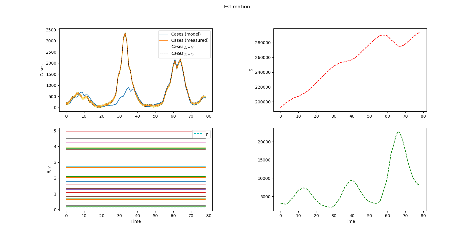
plt.figure(num=1, figsize=(16,8)) plt.suptitle('Estimation') plt.subplot(2,2,1) plt.plot(m.time,m.cases, label='Cases (model)') plt.plot(m.time,cases_meas, label='Cases (measured)') if m.options.EV_TYPE==1:
   plt.plot(m.time,cases_meas+db/2, 'k-.',            linewidth=0.5, label=r'$Cases_{db-hi}$')
   plt.plot(m.time,cases_meas-db/2, 'k-.',            linewidth=0.5, label=r'$Cases_{db-lo}$')
   plt.fill_between(m.time,cases_meas-db/2,                    cases_meas+db/2,color='gold',alpha=.5)
plt.legend(loc='best') plt.ylabel('Cases') plt.subplot(2,2,2) plt.plot(m.time,m.S,'r--') plt.ylabel('S') plt.subplot(2,2,3) [plt.plot(m.time,m.beta[i], label=nolegend) for i in range(nb)] plt.plot(m.time,m.gamma,'c--', label=r'$\gamma$') plt.legend(loc='best') plt.ylabel(r'$\beta, \gamma$') plt.xlabel('Time') plt.subplot(2,2,4) plt.plot(m.time,m.I,'g--') plt.xlabel('Time') plt.ylabel('I') plt.subplots_adjust(hspace=0.2,wspace=0.4)
name = 'cases_EVTYPE_'+ str(m.options.EV_TYPE) + '_gamma' + str(m.gamma.STATUS) + '.png' plt.savefig(name)
- -----------------------------------------------##
- Control
- -----------------------------------------------##
m = m2
m.time = m1.time
- Variables
N = m.FV(value = 3.2e6) mu = m.FV(value = 7.8e-4)
rep_frac = m.FV(value = 0.45)
- beta values (unknown parameters in the model)
beta = [m.FV(value = m1.beta[i].NEWVAL) for i in range(nb)] gamma = m.FV(value = m1.gamma.NEWVAL)
cases = m.CV(value = cases_meas[0],lb=0)
- predicted values
S = m.SV(value=0.06*N, lb=0,ub=N) I = m.SV(value = 0.001*N, lb=0,ub=N)
V = m.CV(value = 2e5) Vr = m.MV(value = 0)
cases.STATUS = 1 cases.FSTATUS = 0 cases.TR_INIT = 0 cases.SPHI = 50 cases.SPLO = 0 cases_SPHI = np.full(len(m.time),cases.SPHI) cases_SPLO = np.full(len(m.time),cases.SPLO)
Vr.STATUS = 1 Vr.UPPER = 1e4 Vr.LOWER = 0 Vr.COST = 1e-5
V.SPHI = 2e5 V.SPLO = 0 V.STATUS = 0 V.TR_INIT = 0 V_SPHI = np.full(len(m.time),V.SPHI) V_SPLO = np.full(len(m.time),V.SPLO)
biweek=[None]*nb for i in range(nb):
biweek[i] = m.Param(value=biweeks[i])
- Intermediates
Rs = m.Intermediate(S*I/N)
- Equations
sum_biweek = sum([biweek[i]*beta[i]*Rs for i in range(nb)]) m.Equation(S.dt()== -sum_biweek + mu*N - Vr) m.Equation(I.dt()== sum_biweek - gamma*I) m.Equation(cases == rep_frac*sum_biweek) m.Equation(V.dt() == -Vr)
- options
m.options.SOLVER = 1
- imode = 6, dynamic control
m.options.IMODE = 6
- ctrl_units = 5, time units are in years
m.options.CTRL_UNITS = 5 m.options.CV_TYPE = 1
- solve model and print solver output
m.solve()
[print('beta[str(i+1)] = '+str(beta[i][0])) for i in range(nb)] print('gamma = '+str(gamma.value[0]))
- export data
- stack time and avg as column vectors
my_data = np.vstack((m.time,np.asarray(beta),V,Vr,gamma))
- transpose data
my_data = my_data.T
- save text file with comma delimiter
beta_str = '' for i in range(nb):
beta_str = beta_str + ',beta[' + str(i+1) + ']'
header_name = 'time,gamma' + beta_str
- np.savetxt('solution_data.csv',my_data,delimiter=',',## header = header_name, comments='')
np.savetxt('solution_control_EVTYPE_str(m.options.EV_TYPE)+ '_gamma'+str(gamma.STATUS).csv', my_data,delimiter=',',header = header_name)
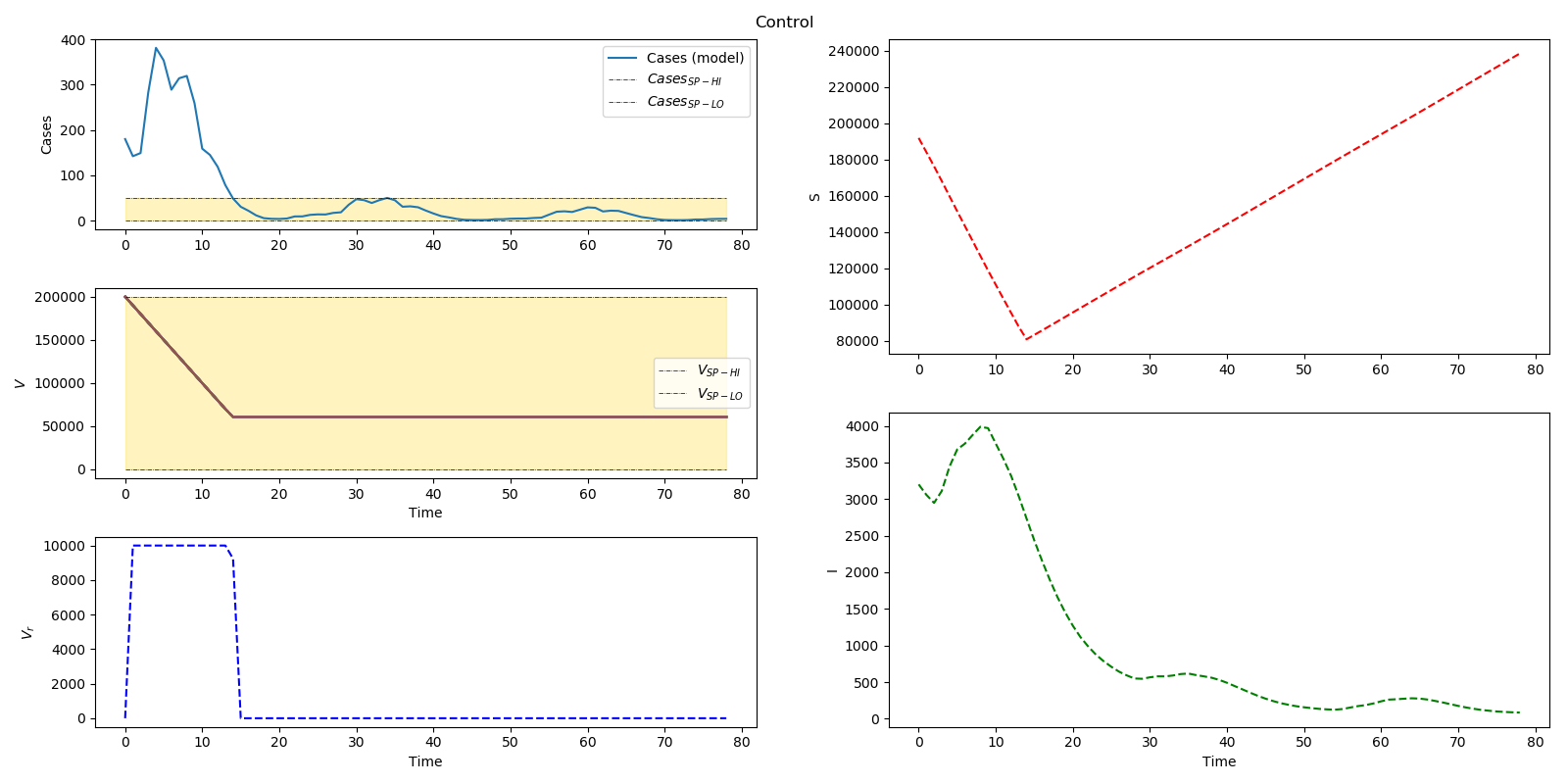
plt.figure(num=2, figsize=(16,8)) plt.suptitle('Control') plt.subplot2grid((6,2),(0,0), rowspan=2) plt.plot(m.time,cases, label='Cases (model)') plt.plot(m.time,cases_SPHI, 'k-.', linewidth=0.5, label=r'$Cases _{SP-HI}$') plt.plot(m.time,cases_SPLO, 'k-.', linewidth=0.5, label=r'$Cases _{SP-LO}$') plt.fill_between(m.time,cases_SPLO,cases_SPHI, color='gold',alpha=.25) plt.legend(loc='best') plt.ylabel('Cases')
plt.subplot2grid((6,2),(0,1), rowspan=3) plt.plot(m.time,S,'r--') plt.ylabel('S')
plt.subplot2grid((6,2),(2,0), rowspan=2) [plt.plot(m.time,V, label=nolegend) for i in range(nb)] plt.plot(m.time,V_SPHI, 'k-.', linewidth=0.5, label=r'$V _{SP-HI}$') plt.plot(m.time,V_SPLO, 'k-.', linewidth=0.5, label=r'$V _{SP-LO}$') plt.fill_between(m.time,V_SPLO,V_SPHI,color='gold',alpha=.25) plt.legend(loc='best') plt.ylabel(r'$V$') plt.xlabel('Time')
plt.subplot2grid((6,2),(3,1),rowspan=3) plt.plot(m.time,I,'g--') plt.xlabel('Time') plt.ylabel('I')
plt.subplot2grid((6,2),(4,0),rowspan=2) plt.plot(m.time,Vr, 'b--') plt.ylabel(r'$V_{r}$') plt.xlabel('Time') plt.tight_layout() plt.subplots_adjust(top=0.95,wspace=0.2) name = 'cases_EVTYPE_'+ str(m.options.EV_TYPE) + '_gamma'+ str(gamma.STATUS) + '.png' plt.savefig(name)
plt.show() (:sourceend:) (:divend:)
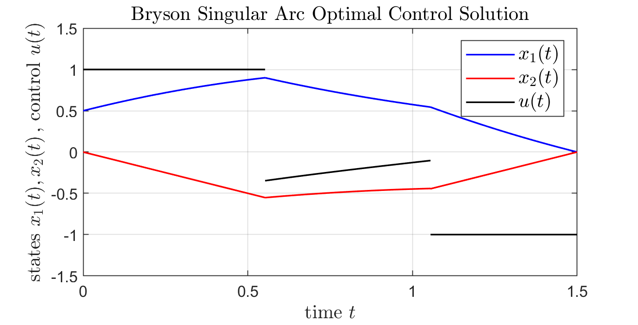
(:toggle hide matlab button show="Show MATLAB Analytic Solution":) (:div id=matlab:) (:source lang=matlab:) % script_BrysonProblem_AnalyticSolution % thanks to Martin Neuenhofen for providing script t0 = 0; tE = 1.5; t1 = 0.5/tanh(1.5);
% t2 is unique solution of % (0.5+t1-0.5*t1^2)*exp(t1-t2)==te-t2+0.5*(tE-t2)^2 % in interval [t0,tE]. t2 = 1.05462;
figure; hold on; box on; axis manual; axis([t0,tE,-1.5,1.5]); grid on;
% interval [t0,t1] u = @(t) 1+0*t; x2 = @(t) -t; x1 = @(t) 0.5+t-0.5*t.^2;
t = linspace(t0,t1,1000); plot(t,x1(t),'blue','linewidth',1); plot(t,x2(t),'red','linewidth',1); plot(t,u(t) ,'black','linewidth',1);
% interval [t1,t2] x1_0 = x1(t1); x2_0 = x2(t1); x1 = @(t) x1_0 ./ exp(t-t1); x2 = @(t) x1_0 * sinh(t-t1) + x2_0 * exp(t-t1); u = @(t) -x1(t)-x2(t);
t = linspace(t1,t2,1000); plot(t,x1(t),'blue','linewidth',1); plot(t,x2(t),'red','linewidth',1); plot(t,u(t) ,'black','linewidth',1);
% interval [t2,tE] u = @(t) -1+0*t; x2 = @(t) -1.5+t; x1 = @(t) (tE-t)+0.5*(tE-t).^2;
t = linspace(t2,tE,1000); plot(t,x1(t),'blue','linewidth',1); plot(t,x2(t),'red','linewidth',1); plot(t,u(t) ,'black','linewidth',1);
legend({'$x_1(t)$','$x_2(t)$','$u(t)$'},...
'Interpreter','LateX','fontsize',12);
title('Bryson Singular Arc Optimal Control Solution',...
'Interpreter','LateX','fontsize',12);
xlabel('time $t$','Interpreter','LateX','fontsize',12); ylabel('states $x_1(t),x_2(t)$\,, control $u(t)$',...
'Interpreter','LateX','fontsize',12);
(:sourceend:) (:divend:)
(:toggle hide gekko2 button show="Show GEKKO (Python) Code":) (:div id=gekko2:) (:source lang=python:) from gekko import GEKKO import numpy as np import matplotlib.pyplot as plt
- Build Model ############################
m = GEKKO()
- define time space
nt = 101 m.time = np.linspace(0,1.5,nt)
- Parameters
u = m.MV(value =0, lb = -1, ub = 1) u.STATUS = 1 u.DCOST = 0.0001 # slight penalty to discourage MV movement
- Variables
x1 = m.Var(value=0.5) x2 = m.Var(value = 0) myObj = m.Var()
- Equations
m.Equation(myObj.dt() == 0.5*x1**2) m.Equation(x1.dt() == u + x2) m.Equation(x2.dt() == -u)
f = np.zeros(nt) f[-1] = 1 final = m.Param(value=f)
- Four options for final constraints x1(tf)=0 and x2(tf)=0
option = 2 # best option = 3 (fix endpoints directly) if option == 1:
    # most likely to cause DOF issues because of many 0==0 equations
    m.Equation(final*x1 == 0)
    m.Equation(final*x2 == 0)
elif option == 2:
    # inequality constraint approach is better but there are still
    #   many inactive equations not at the endpoint
    m.Equation((final*x1)**2 <= 0)
    m.Equation((final*x2)**2 <= 0)
elif option == 3: #requires GEKKO version >= 0.0.3a2
    # fix the value just at the endpoint (best option)
    m.fix(x1,nt-1,0)
    m.fix(x2,nt-1,0)
else:
    #penalty method ("soft constraint") that may influence the
    # optimal solution because there is just one combined objective
    # and it may interfere with minimizing myObj
    m.Obj(1000*(final*x1)**2)
    m.Obj(1000*(final*x2)**2)
m.Obj(myObj*final)
- Set Global Options and Solve
m.options.IMODE = 6 m.options.NODES = 3 m.options.MV_TYPE = 1 m.options.SOLVER = 1 # APOPT solver
- Solve
m.solve() # (remote=False) for local solution
- Print objective value
print('Objective (myObj): ' + str(myObj[-1]))
- Plot Results
plt.figure() plt.plot(m.time, x1.value, 'y:', label = '$x_1$') plt.plot(m.time, x2.value, 'r--', label = '$x_2$') plt.plot(m.time, u.value, 'b-', label = 'u') plt.plot(m.time, myObj.value,'k-',label='Objective') plt.legend() plt.show() (:sourceend:) (:divend:)
<iframe width="560" height="315" src="https://www.youtube.com/embed/UTTlZ6rVXxM" frameborder="0" allowfullscreen></iframe>
<iframe width="560" height="315" src="https://www.youtube.com/embed/0CWkV2TMO6U" frameborder="0" allowfullscreen></iframe>
Problem 1 Solution (Orthogonal Collocation)
(:html:) <iframe width="560" height="315" src="https://www.youtube.com/embed/giShP5WNqiw" frameborder="0" allowfullscreen></iframe> (:htmlend:)
Problem 2 Solution (Bryson Benchmark)
(:html:) (:htmlend:)
Problem 3 Solution (Infectious Disease)
(:html:) (:htmlend:)
(:title Midterm Exam for Dynamic Optimization:) (:keywords Python, MATLAB, Simulink, nonlinear control, model predictive control, exam, midterm:) (:description Mid-term exam for dynamic estimation and optimization as a graduate-level course.:)