Dynamic Optimization

m.Maximize(Jf)

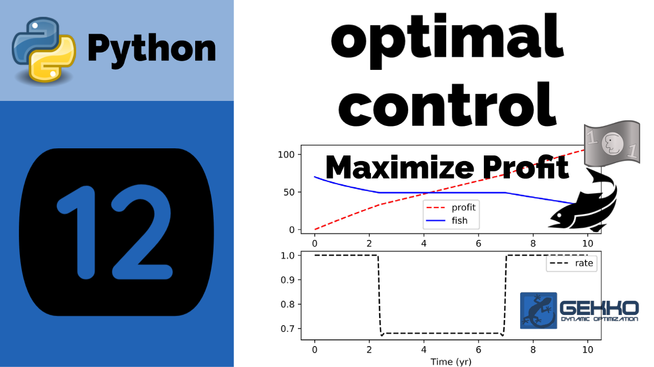
The commercial fishing optimal control problem has an integral profit function that includes the cost of operations and the revenue from fish sales. The population of fish x is influenced by how many fish are removed each year that depends on u. The objective is to maximize the revenue from fishing over a 10 year time period. If there is overfishing (high u) then the returns for subsequent years are reduced and the fish population does not recover. This optimal control problem finds the optimal extraction profile to maximize the commercial fishing profit.

<iframe width="560" height="315" src="https://www.youtube.com/embed/y26X-BSf8KU" frameborder="0" allow="autoplay; encrypted-media" allowfullscreen></iframe>

Integrals are a natural expression of many systems where the accumulation of a quantity is maximized or minimized. The integral is the profit function over the 10 year time period.

$$\max_{u(t)} \int_0^{10} \left(E-\frac{c}{x}\right) u \, U_{max} \, dt$$ $$\mathrm{subject \; to}$$ $$\frac{dx}{dt}=r \, x(t) \left(1-\frac{x(t)}{k}\right)-u \, U_{max}$$ $$x(0) = 70$$ $$0 \le u(t) \le 1$$ $$E=1, \, c=17.5, \, r=0.71, \, k=80.5, \, U_{max}=20$$

Integral expressions are reformulated in differential and algebraic form by defining a new variable.

$$J = \int_0^{10} \left(E-\frac{c}{x}\right) u \, U_{max} \, dt$$

The new variable J and integral are differentiated and included as an additional equation. The problem then becomes a maximization of the new variable J at the final time.

$$\max_{u(t)} J\left(t_f\right)$$ $$\mathrm{subject \; to}$$ $$\frac{dx}{dt}=r \, x(t) \left(1-\frac{x(t)}{k}\right)-u \, U_{max}$$ $$\frac{dJ}{dt} = \left(E-\frac{c}{x}\right) u \, U_{max}$$ $$x(0) = 70$$ $$J(0) = 0$$ $$0 \le u(t) \le 1$$ $$t_f = 10, \, E=1, \, c=17.5, \, r=0.71, \, k=80.5, \, U_{max}=20$$

The initial condition of the integral J starts at zero and becomes the integral in the time range of 0 to 10. The end value is maximized at the final point in the time horizon of the optimal control problem. A maximization problem is converted to a minimization problem by multiplying the objective by negative one.

$$\max_{u(t)} J\left(t_f\right) = -\min_{u(t)} J\left(t_f\right)$$

Most optimization solvers require an objective function minimization, including GEKKO and APMonitor.

Solutions in APM MATLAB and APM Python

Economic Optimization of Fishery in MATLAB and Python

<iframe width="560" height="315" src="https://www.youtube.com/embed/MA53XPp-a7I" frameborder="0" allowfullscreen></iframe>

(:title Economic Model Predictive Control (MPC):)

Most optimization solvers require an objective function minimization, including GEKKO and APMonitor.

from gekko import GEKKO import numpy as np import matplotlib.pyplot as plt

1. create GEKKO model

m = GEKKO()

1. time points

n=501 m.time = np.linspace(0,10,n)

1. constants

E = 1 c = 17.5 r = 0.71 k = 80.5 U_max = 20

1. fishing rate

u = m.MV(value=1,lb=0,ub=1) u.STATUS = 1 u.DCOST = 0

1. fish population

x = m.Var(value=70)

1. fish population balance

m.Equation(x.dt() == r*x*(1-x/k)-u*U_max)

1. objective (profit)

J = m.Var(value=0)

1. final objective

Jf = m.FV() Jf.STATUS = 1 m.Connection(Jf,J,pos2='end') m.Equation(J.dt() == (E-c/x)*u*U_max)

1. maximize profit

m.Obj(-Jf)

1. options

m.options.IMODE = 6 # optimal control m.options.NODES = 3 # collocation nodes m.options.SOLVER = 3 # solver (IPOPT)

1. solve optimization problem

m.solve()

1. print profit

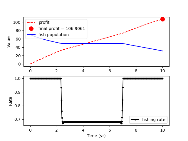
print('Optimal Profit: ' + str(Jf.value[0]))

1. plot results

plt.figure(1) plt.subplot(2,1,1) plt.plot(m.time,J.value,'r--',label='profit') plt.plot(m.time[-1],Jf.value[0],'ro',markersize=10, label='final profit = '+str(Jf.value[0])) plt.plot(m.time,x.value,'b-',label='fish population') plt.ylabel('Value') plt.legend() plt.subplot(2,1,2) plt.plot(m.time,u.value,'k.-',label='fishing rate') plt.ylabel('Rate') plt.xlabel('Time (yr)') plt.legend() plt.show()

$$E=1, \, c=17.5, \, r=0.71, \, k=80.5, \, U_{max}=20$$

$$t_f = 10, \, E=1, \, c=17.5, \, r=0.71, \, k=80.5, \, U_{max}=20$$

$$\max_{u(t)} \int_0^{10} \left(E-\frac{c}{x}\right) u \, U_{max} \, dt$$

$$J = \int_0^{10} \left(E-\frac{c}{x}\right) u \, U_{max} \, dt$$

(:title Economic Optimization of Fishing:)

The commercial fishing optimal control problem has an integral objective function. The population of fish x is influenced by how many fish are removed each year that depends on u. The objective is to maximize the revenue from fishing over a 10 year time period. If there is overfishing (high u) then the returns for subsequent years are reduced and the fish population does not recover. This optimal control problem finds the optimal extraction profile to maximize the commercial fishing profit.

Integrals are a natural expression of many systems where the accumulation of a quantity is maximized or minimized. The integral is the profit function over the 10 year time period.

(:title Economic Optimization of Commercial Fishing:) (:keywords nonlinear control, fishing, optimal control, dynamic optimization, sustainability, MATLAB, Python, GEKKO, optimization suite:) (:description Economic optimization using model forecasts for harvesting and supply. The problem is solved with MATLAB, Python, and GEKKO.:)

Objective: Set up and solve the commercial fishing economic optimal control problem. Create a program to optimize and display the results. Estimated Time: 30 minutes

The commercial fishing optimal control problem has an integral objective function. Integrals are a natural expression of many systems where the accumulation of a quantity is maximized or minimized.

$$\max_{u(t)} \int_0^10 \left(E-\frac{c}{x}\right) u \, U_{max} \, dt$$ $$\mathrm{subject \; to}$$ $$\frac{dx}{dt}=r \, x(t) \left(1-\frac{x(t)}{k}\right)-u \, U_{max}$$ $$x(0) = 70$$ $$0 \le u(t) \le 1$$ $$E=1, \, c=17.5 \, r=0.71 \, k=80.5 \, U_{max}=20$$

Integral expressions are reformulated in differential and algebraic form by defining a new variable.

$$J = \int_0^10 \left(E-\frac{c}{x}\right) u \, U_{max} \, dt$$

The new variable J and integral are differentiated and included as an additional equation. The problem then becomes a maximization of the new variable J at the final time.

$$\max_{u(t)} J\left(t_f\right)$$ $$\mathrm{subject \; to}$$ $$\frac{dx}{dt}=r \, x(t) \left(1-\frac{x(t)}{k}\right)-u \, U_{max}$$ $$\frac{dJ}{dt} = \left(E-\frac{c}{x}\right) u \, U_{max}$$ $$x(0) = 70$$ $$J(0) = 0$$ $$0 \le u(t) \le 1$$ $$t_f = 10, \, E=1, \, c=17.5 \, r=0.71 \, k=80.5 \, U_{max}=20$$

The initial condition of the integral J starts at zero and becomes the integral in the time range of 0 to 10. The end value is maximized at the final point in the time horizon of the optimal control problem. A maximization problem is converted to a minimization problem by multiplying the objective by negative one.

$$\max_{u(t)} J\left(t_f\right) = -\min_{u(t)} J\left(t_f\right)$$

Most optimization solvers require an objective function minimization.

Solutions

Economic Optimization of Fishery in MATLAB and Python

(:html:) <iframe width="560" height="315" src="https://www.youtube.com/embed/MA53XPp-a7I" frameborder="0" allowfullscreen></iframe> (:htmlend:)

(:toggle hide gekko button show="GEKKO (Python) Solution":) (:div id=gekko:) (:source lang=python:) (:sourceend:) (:divend:)

(:html:) (:htmlend:)

References

1. Beal, L., GEKKO for Dynamic Optimization, 2018, URL: https://gekko.readthedocs.io/en/latest/
2. Hedengren, J. D. and Asgharzadeh Shishavan, R., Powell, K.M., and Edgar, T.F., Nonlinear Modeling, Estimation and Predictive Control in APMonitor, Computers and Chemical Engineering, Volume 70, pg. 133–148, 2014. Article