Dynamic Control Introduction
Main.DynamicControl History
Show minor edits - Show changes to markup
import matplotlib.pyplot as plt
- constants
- Parameters
- Manipulated variable
- Controlled Variable
p.STATUS = 1 # allow optimizer to change p.DCOST = 0.1 # smooth out gas pedal movement p.DMAX = 20 # slow down change of gas pedal
v.STATUS = 1 # add the SP to the objective m.options.CV_TYPE = 2 # sq error v.SP = 40 # set point v.TR_INIT = 1 # setpoint trajectory v.TAU = 5 # time constant of setpoint trajectory
m.options.IMODE = 6 #control
m.options.IMODE = 6 #control
- MV tuning
p.STATUS = 1 #allow optimizer to change p.DCOST = 0.1 #smooth out gas pedal movement p.DMAX = 20 #slow down change of gas pedal
- CV tuning
- setpoint
v.STATUS = 1 #add the SP to the objective m.options.CV_TYPE = 2 #L2 norm v.SP = 40 #set point v.TR_INIT = 1 #setpoint trajectory v.TAU = 5 #time constant of setpoint trajectory
- Solve
import matplotlib.pyplot as plt
plt.ylabel('velocity') plt.xlabel('time')
plt.ylabel('velocity'); plt.xlabel('time')

(:toggle hide gekko button show="Show GEKKO (Python) Code":) (:div id=gekko:)
Model Predictive Control is solved repeatedly at a specified cycle time as new measurements arrive or a new setpoint is specified. The model is updated with initial conditions from the next time step and the horizon is extended by an additional time unit to maintain a constant time horizon for predictive control.
(:toggle hide gekko2 button show="Show GEKKO (Python) Code":) (:div id=gekko2:)
- Import packages
from random import random
- Build model
- initialize GEKKO model
- time
- Equations
- Tuning
- global
(:toggle hide gekko button show="Show GEKKO (Python) Code":) (:div id=gekko:) (:source lang=python:) import numpy as np from gekko import GEKKO import matplotlib.pyplot as plt from PIL import Image
- Initialize the GEKKO model
m = GEKKO(remote=False) m.time = np.linspace(0, 20, 21) # Time grid mass = 500 b = m.Param(value=50) K = m.Param(value=0.8) p = m.MV(value=0, lb=0, ub=100) # Manipulated Variable (gas pedal) v = m.CV(value=0) # Controlled Variable (velocity)
- Define the dynamic equation
m.Equation(mass * v.dt() == -v * b + K * b * p)
- Set optimization mode for control
m.options.IMODE = 6 # Control mode
- Tuning parameters for MV (gas pedal)
p.STATUS = 1 # Allow optimizer to change p.FSTATUS = 0 p.DCOST = 0.1 # Smooth out gas pedal movement p.DMAX = 20 # Limit rate of change
- Tuning parameters for CV (velocity)
v.STATUS = 1 # Include set point in the objective m.options.CV_TYPE = 2 # L2 norm v.SP = 40 # Set point for velocity v.TR_INIT = 1 # Enable set point trajectory v.TAU = 5 # Time constant of trajectory
- List to store frames for GIF
frames = []
- Run the optimization in a loop and save plots
for i in range(25):
    if i==15:
        v.SP = 20

    print(f'MPC cycle: {i} of 25')
    m.solve(disp=False)  # Solve the optimization problem

    # Create a plot for each iteration
    fig, (ax1, ax2) = plt.subplots(2, 1, figsize=(6, 8))

    ax1.plot(m.time+i, p.value, 'b-', lw=2)
    ax1.set_ylabel('Gas Pedal (%)')
    ax1.set_title(f'MPC Cycle {i+1}')
    ax1.set_ylim([0,100])

    ax2.plot(m.time+i, v.value, 'r--', lw=2)
    ax2.plot(m.time+i,np.ones_like(m.time)*v.SP,'k:',lw=2)
    ax2.set_ylim([0,50])
    ax2.set_ylabel('Velocity (m/s)')
    ax2.set_xlabel('Time (s)')
    fig.tight_layout()

    # Save the plot as an image frame
    fig.canvas.draw()
    frame = np.frombuffer(fig.canvas.tostring_rgb(), dtype='uint8')
    frame = frame.reshape(fig.canvas.get_width_height()[::-1] + (3,))
    frames.append(Image.fromarray(frame))

    plt.close(fig)  # Close the figure to save memory
- Save the frames as a GIF
frames[0].save('control_simulation.gif', format='GIF',
append_images=frames[1:], save_all=True, duration=500, loop=0)
print("GIF saved as 'control_simulation.gif'") (:sourceend:) (:divend:)
- The first step to solve a model predictive control (MPC) in Python Gekko is to define the MPC problem. This may involve setting the time horizon and decision variables, constraints, objective function, and other parameters.
- Once the problem is defined, the next step is to create the MPC object. This is done by setting m.options.IMODE=6. The parameters of the MPC object can be set in m.options.
- The third step is to solve the MPC problem. This is done by calling the m.solve() command. This will solve the MPC problem and return the optimal solution.
- The fourth step is to process the solution. This can involve extracting the optimal decisions, evaluating the objective function, and other processing steps.
- Finally, the fifth step is to apply the optimal decisions. This can involve setting the plant state or inputs based on the optimal decisions.
plt.plot(m.time,p.value,'b-',LineWidth=2)
plt.plot(m.time,p.value,'b-',lw=2)
plt.plot(m.time,v.value,'r--',LineWidth=2)
plt.plot(m.time,v.value,'r--',lw=2)
(:toggle hide gekko button show="Show GEKKO (Python) Code":) (:div id=gekko:) (:source lang=python:)
- Import packages
import numpy as np from random import random from gekko import GEKKO import matplotlib.pyplot as plt
- Build model
- initialize GEKKO model
m = GEKKO()
- time
m.time = np.linspace(0,20,41)
- constants
mass = 500
- Parameters
b = m.Param(value=50) K = m.Param(value=0.8)
- Manipulated variable
p = m.MV(value=0, lb=0, ub=100)
- Controlled Variable
v = m.CV(value=0)
- Equations
m.Equation(mass*v.dt() == -v*b + K*b*p)
- Tuning
- global
m.options.IMODE = 6 #control
- MV tuning
p.STATUS = 1 #allow optimizer to change p.DCOST = 0.1 #smooth out gas pedal movement p.DMAX = 20 #slow down change of gas pedal
- CV tuning
- setpoint
v.STATUS = 1 #add the SP to the objective m.options.CV_TYPE = 2 #L2 norm v.SP = 40 #set point v.TR_INIT = 1 #setpoint trajectory v.TAU = 5 #time constant of setpoint trajectory
- Solve
m.solve()
- Plot solution
plt.figure() plt.subplot(2,1,1) plt.plot(m.time,p.value,'b-',LineWidth=2) plt.ylabel('gas') plt.subplot(2,1,2) plt.plot(m.time,v.value,'r--',LineWidth=2) plt.ylabel('velocity') plt.xlabel('time') plt.show() (:sourceend:) (:divend:)
Objective: Implement a model predictive controller that automatically regulates vehicle velocity. Implement the controller in Excel, MATLAB, Python, or Simulink and tune the controller for acceptable performance. Discuss factors that may be import for evaluating controller performance. Estimated time: 1 hour
Objective: Implement a model predictive controller that automatically regulates vehicle velocity. Implement the controller in Excel, MATLAB, Python, or Simulink and tune the controller for acceptable performance. Discuss factors that may be important for evaluating controller performance. Estimated time: 1 hour
Objective: Implement a model predictive controller that automatically regulates vehicle velocity. Implement the controller in MATLAB, Python, and Simulink and tune the controller for acceptable performance. Discuss factors that may be import for evaluating controller performance. Estimated time: 2 hours
Objective: Implement a model predictive controller that automatically regulates vehicle velocity. Implement the controller in Excel, MATLAB, Python, or Simulink and tune the controller for acceptable performance. Discuss factors that may be import for evaluating controller performance. Estimated time: 1 hour
- The dynamic relationship between a vehicle gas pedal position (MV) and velocity (CV) is given by the following set of conditions and a single dynamic equation.
The dynamic relationship between a vehicle gas pedal position (MV) and velocity (CV) is given by the following set of conditions and a single dynamic equation.
- Discuss the controller performance and how it could be tuned to meet multiple objectives including:
Discuss the controller performance and how it could be tuned to meet multiple objectives including:
A method to solve dynamic control problems is by numerically integrating the dynamic model at discrete time intervals, much like measuring a physical system at particular time points. The numerical solution is compared to a desired trajectory and the difference is minimized by adjustable parameters in the model that may change at every time step. The first control action is taken and then the entire process is repeated at the next time instance. The process is repeated because objective targets may change or updated measurements may have adjusted parameter or state estimates. Excel, MATLAB, Python, and Simulink are used in the following example to both solve the differential equations that describe the velocity of a vehicle as well as minimize the control objective function.
A method to solve dynamic control problems is by numerically integrating the dynamic model at discrete time intervals, much like measuring a physical system at particular time points. The numerical solution is compared to a desired trajectory and the difference is minimized by adjustable parameters in the model that may change at every time step. The first control action is taken and then the entire process is repeated at the next time instance. The process is repeated because objective targets may change or updated measurements may have adjusted parameter or state estimates.
Exercise
Objective: Implement a model predictive controller that automatically regulates vehicle velocity. Implement the controller in MATLAB, Python, and Simulink and tune the controller for acceptable performance. Discuss factors that may be import for evaluating controller performance. Estimated time: 2 hours
- The dynamic relationship between a vehicle gas pedal position (MV) and velocity (CV) is given by the following set of conditions and a single dynamic equation.
 Constants
   m = 500 ! Mass (kg)
 Parameters
   b = 50  ! Resistive coefficient (N-s/m)
   K = 0.8 ! Gain (m/s-%pedal)
   p = 0 >= 0 <= 100  ! Gas pedal position (%)
 Variables
   v = 0 ! initial condition
 Equations
   m * $v = -v * b + K * b * p
Implement a model predictive controller that adjusts gas pedal position to regulate velocity. Start at an initial vehicle velocity of 0 m/s and accelerate to a velocity of 40 m/s.
- Discuss the controller performance and how it could be tuned to meet multiple objectives including:
- minimize travel time
- remain within speed limits
- improve vehicle fuel efficiency
- discourage excessive gas pedal adjustments
- do not accelerate excessively
There is no need to implement these advanced objectives in simulation for this second part of the exercise, only discuss the possible competing objectives.
Solution
Excel, MATLAB, Python, and Simulink are used in this example to both solve the differential equations that describe the velocity of a vehicle as well as minimize the control objective function.
Exercise
Objective: Set up and solve several dynamic optimization benchmark problems1. Create a program to optimize and display the results. Estimated Time (each): 30 minutes
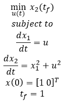
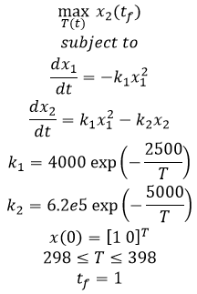
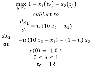
- Example 1a - Nonlinear, unconstrained, minimize final state
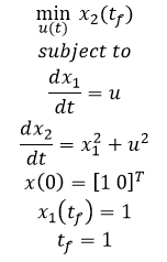
- Example 1b - Nonlinear, unconstrained, minimize final state with terminal constraint
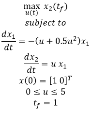
- Example 2 - Nonlinear, constrained, minimize final state
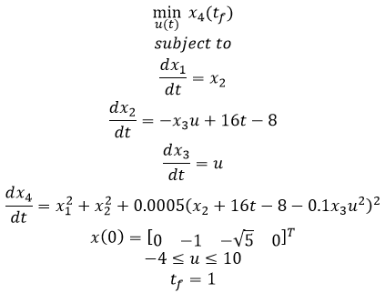
- Example 3 - Tubular reactor with parallel reaction
- Example 4 - Batch reactor with consecutive reactions A->B->C
Example 5 - Catalytic plug flow reactor with A->B->C
Solution

References
- M. Čižniar, M. Fikar, M.A. Latifi: A MATLAB Package for Dynamic Optimisation of Processes, 7th International Scientific – Technical Conference – Process Control 2006, June 13 – 16, 2006, Kouty nad Desnou, Czech Republic. Article
Objective: Set up and solve several dynamic optimization benchmark problems1. Create a program to optimize and display the results. Estimated Time (each): 30 minutes
Objective: Set up and solve several dynamic optimization benchmark problems1. Create a program to optimize and display the results. Estimated Time (each): 30 minutes
- M. Čižniar, M. Fikar, M.A. Latifi: A MATLAB Package for Dynamic Optimisation of Processes, 7th International Scientific – Technical Conference – Process Control 2006, June 13 – 16, 2006, Kouty nad Desnou, Czech Republic.
- M. Čižniar, M. Fikar, M.A. Latifi: A MATLAB Package for Dynamic Optimisation of Processes, 7th International Scientific – Technical Conference – Process Control 2006, June 13 – 16, 2006, Kouty nad Desnou, Czech Republic. Article
Exercise
Objective: Set up and solve several dynamic optimization benchmark problems1. Create a program to optimize and display the results. Estimated Time (each): 30 minutes
- Example 1a - Nonlinear, unconstrained, minimize final state
- Example 1b - Nonlinear, unconstrained, minimize final state with terminal constraint
- Example 2 - Nonlinear, constrained, minimize final state
- Example 3 - Tubular reactor with parallel reaction
- Example 4 - Batch reactor with consecutive reactions A->B->C
Example 5 - Catalytic plug flow reactor with A->B->C
Solution
References
- M. Čižniar, M. Fikar, M.A. Latifi: A MATLAB Package for Dynamic Optimisation of Processes, 7th International Scientific – Technical Conference – Process Control 2006, June 13 – 16, 2006, Kouty nad Desnou, Czech Republic.
<iframe width="560" height="315" src="https://www.youtube.com/embed/umxAfu44kWo?rel=0" frameborder="0" allowfullscreen></iframe>
<iframe width="560" height="315" src="https://www.youtube.com/embed/dqm2OqXYLR8?rel=0" frameborder="0" allowfullscreen></iframe>
(:html:) <iframe width="560" height="315" src="https://www.youtube.com/embed/DFqOf5wbQtc?rel=0" frameborder="0" allowfullscreen></iframe> (:htmlend:)
Dynamic control is a method to use model predictions to plan an optimized future trajectory for time-varying systems. It is often referred to as Model Predictive Control (MPC) or Dynamic Optimization.
Dynamic control is a method to use model predictions to plan an optimized future trajectory for time-varying systems. It is often referred to as Model Predictive Control (MPC) or Dynamic Optimization.
Model Predictive Control Example
A method to solve dynamic control problems is by numerically integrating the dynamic model at discrete time intervals, much like measuring a physical system at particular time points. The numerical solution is compared to a desired trajectory and the difference is minimized by adjustable parameters in the model that may change at every time step. The first control action is taken and then the entire process is repeated at the next time instance. The process is repeated because objective targets may change or updated measurements may have adjusted parameter or state estimates. Excel, MATLAB, Python, and Simulink are used in the following example to both solve the differential equations that describe the velocity of a vehicle as well as minimize the control objective function.
(:html:) <iframe width="560" height="315" src="https://www.youtube.com/embed/umxAfu44kWo?rel=0" frameborder="0" allowfullscreen></iframe> (:htmlend:)
(:title Dynamic Control Introduction:) (:keywords control, dynamics, dynamic optimization, simulation, modeling language, differential, algebraic, tutorial:) (:description Dynamic control in MATLAB and Python for use in real-time or off-line applications:)
Dynamic control is a method to use model predictions to plan an optimized future trajectory for time-varying systems. It is often referred to as Model Predictive Control (MPC) or Dynamic Optimization.