Objective: Quantify the TCLab offset between the setpoint (desired target) and the measured temperature when using a proportional-only controller.

A proportional only (P-only) controller is the simplest implementation of a PID controller without the integral or derivative terms. The controller is an equation that adjusts the controller output, `u(t)`, for input into the system as the manipulated variable. It is a calculation of the difference between the setpoint SP and process variable PV. The adjustable parameter is the controller gain, `K_c`. A large gain produces a controller that reacts aggressively to a difference between the measured PV and target SP.

$$Q(t) = Q_{bias} + K_c \, \left( T_{SP}-T_{PV} \right) = Q_{bias} + K_c \, e(t)$$

The `Q_{bias}` term is a constant that is typically set to the value of `Q(t)` when the controller is first switched from manual to automatic mode. The deviation variable for the heater is the change in value `Q'(t) = Q(t) - Q_{bias}`. For the TCLab, `Q_{bias}`=0 because the TCLab starts with the heater off. The `Q_{bias}` gives bumpless transfer if the error is zero when the controller is turned on. The error from the set point is the difference between the `T_{SP}` and `T_{PV}` and is defined as `e(t) = T_{SP} - T_{PV}`. See additional information on P-only controllers.

The TCLab is a non-integrating process because the temperature returns to ambient conditions when the heater is shut off. A P-only controller has persistent offset between the SP and PV at steady-state for non-integrating systems. The purpose of this assignment is to calculate and then verify the offset for the TCLab.

A common tuning correlation for P-only control is the ITAE (Integral of Time-weighted Absolute Error) method. Use the ITAE setpoint tracking tuning correlation with FOPDT parameters (`K_c`, `\tau_p`, `\theta_p`) determined from the TCLab graphical fitting or TCLab regression exercises.

$$K_c = \frac{0.20}{K_p}\left(\frac{\tau_p}{\theta_p}\right)^{1.22} \quad \mathrm{Set\;point\;tracking}$$

P-Only Offset Simulator

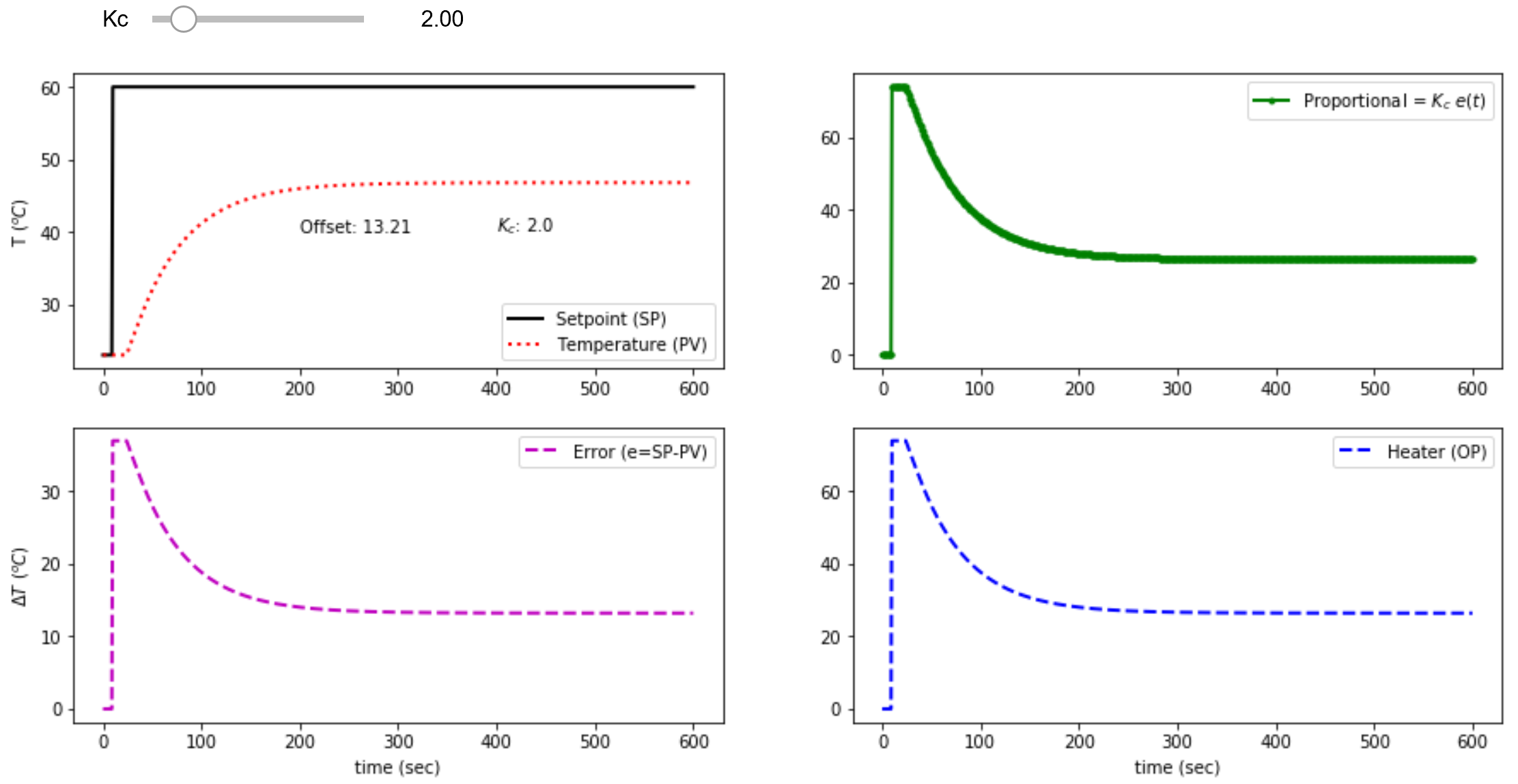
Use the P-Only offset simulator to test the control performance before implementing on the TCLab. The simulator shows the offset for a TCLab FOPDT model with `K_p`=0.9 ^oC/%, `\tau_p`=175.0 sec, and `\theta_p`=15.0 sec. Use the FOPDT model parameters for your own TCLab device for a more accurate estimate of offset. The controller gain `K_c` is adjusted with a slider to compute the updated offset values as shown on the plot.

GitHub Colab

P-Only Control with TCLab

Fill in the value of `K_c` and the P-only equation in the code below and run with the TCLab to experimentally determine the offset from a step in setpoint from 23^oC to 60^oC.

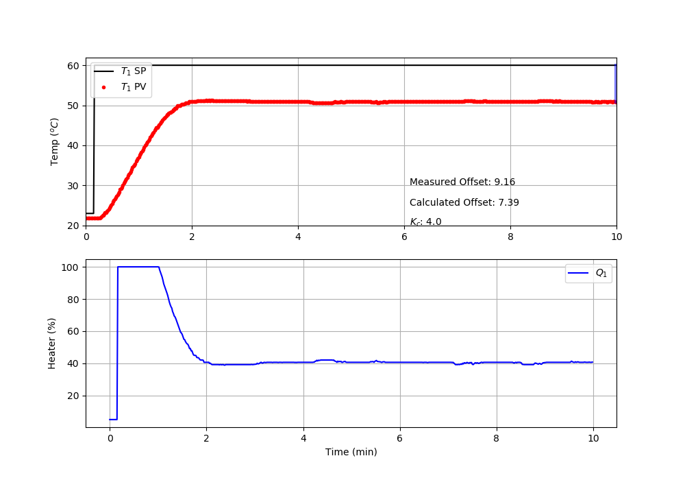
Calculate the predicted offset from the FOPDT model. In the solution, include a plot of the P-only controller response. Indicate the measured and calculated offset values graphically on the plot.

Solution

The predicted offset is calculated from the FOPDT model and P-only controller equation.

$$\tau_p \frac{dT'}{dt} = -T' + K_p \, Q'\left(t-\theta_p\right)$$

At steady-state the model becomes:

$$0 = -(T-23) + K_p \, Q'$$

The control output is:

$$Q' = K_c \left(60-T\right)$$

These two equations are combined to solve for `T`:

$$T=\frac{23+K_p\,K_c\,60}{1+K_p\,K_c}$$

and offset=`(60-T)`:

$$\mathrm{offset} = 60-T = 60 - \frac{23+K_p\,K_c\,60}{1+K_p\,K_c}$$

$$\mathrm{offset} = 60-T = 60 - \frac{23+0.9 \times 4.45 \times 60}{1+0.9 \times 4.45}$$

$$\mathrm{offset} = 60-T = 60 - 52.6 = 7.4^oC$$

The plot of the P-only controller response shows a similar offset (`9.1^oC`) to the calculated value (`7.4^oC`).

import numpy as np
import matplotlib.pyplot as plt
import tclab
import time

# -----------------------------
# Adjust controller gain (Kc)
#  from ITAE tuning correlation
# -----------------------------
Kc = 4.45

n = 600  # Number of second time points (10 min)
tm = np.linspace(0,n-1,n) # Time values
lab = tclab.TCLab()
T1 = np.zeros(n)
Q1 = np.zeros(n)
# step setpoint from 23.0 to 60.0 degC
SP1 = np.ones(n)*23.0
SP1[10:] = 60.0
Q1_bias = 0.0
for i in range(n):
    # record measurement
    T1[i] = lab.T1

    # --------------------------------------------------
    # fill-in P-only controller equation to change Q1[i]
    # --------------------------------------------------
    Q1[i] = Q1_bias + Kc * (SP1[i]-T1[i])

    # implement new heater value
    Q1[i] = max(0,min(100,Q1[i])) # clip to 0-100%
    lab.Q1(Q1[i])
    if i%20==0:
        print(' Heater,   Temp,  Setpoint')
    print(f'{Q1[i]:7.2f},{T1[i]:7.2f},{SP1[i]:7.2f}')
    # wait for 1 sec
    time.sleep(1)
lab.close()
# Save data file
data = np.vstack((tm,Q1,T1,SP1)).T
np.savetxt('P-only.csv',data,delimiter=',',\
           header='Time,Q1,T1,SP1',comments='')

# Create Figure
plt.figure(figsize=(10,7))
ax = plt.subplot(2,1,1)
ax.grid()
plt.plot(tm/60.0,SP1,'k-',label=r'$T_1$ SP')
plt.plot(tm/60.0,T1,'r.',label=r'$T_1$ PV')
plt.text(6.1,30,'Measured Offset: ' + str(np.round(SP1[-1]-T1[-1],2)))
offset = 60 - (23+0.9*Kc*60)/(1+0.9*Kc)
plt.text(6.1,26,'Calculated Offset: ' + str(np.round(offset,2)))
plt.text(6.1,22,r'$K_c$: ' + str(np.round(Kc,2)))  
plt.plot([tm[-1]/60.0,tm[-1]/60.0],[SP1[-1],T1[-1]],\
         'b-',lw=3,alpha=0.5)
plt.ylabel(r'Temp ($^oC$)')
plt.xlim([0,10])
plt.legend(loc=2)
ax = plt.subplot(2,1,2)
ax.grid()
plt.plot(tm/60.0,Q1,'b-',label=r'$Q_1$')
plt.ylabel(r'Heater (%)')
plt.xlabel('Time (min)')
plt.legend(loc=1)
plt.savefig('P-only_Control.png')
plt.show()

[$[Get Code]]

Generative AI Learning

Use these prompts to test your understanding after completing the exercise. Direct the AI - do not let it do the exercise for you.

App: Run P-only experiments safely in the browser with the TCLab Control Studio - set tau-I very large (or integral off) in the PID panel to get P-only action, try several Kc values on the digital twin, and export the CSV for your report.

What to Turn In

Submit a short report (PDF, 1-2 pages) that curates your results into a demonstration of what you learned. You may use Generative AI to help write the report, but you must guide it to the correct visualizations, justifications, and assumptions. Answer these questions:

1. Include plots of setpoint, temperature, and heater output for at least two Kc values. Report the steady-state offset for each.
2. Compare the measured offsets to the predicted offset formula using your FOPDT Kp. How close are they, and what explains the gap?
3. What Kc would be needed to cut the offset to 1 degC, and why is simply raising Kc not a good strategy on a real process?
4. From the quiz prompt: one question you missed and the corrected answer.