Consider a cylindrical tank with no outlet flow and an adjustable inlet flow that is controlled by a valve. The inlet flow rate is not measured but there is a level measurement that shows how much fluid has been added to the tank. The objective of this exercise is to develop a controller that can maintain a certain water level by automatically adjusting the inlet flow rate.

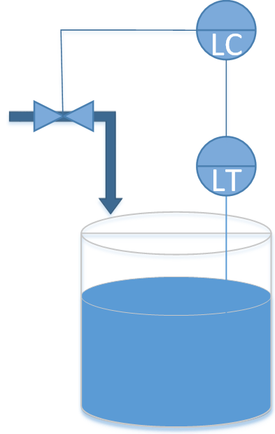
Note: The symbol LT is an abbreviation for Level Transmitter. A concentration sensor is typically shown as CT for Concentration Transmitter or AT for Analyzer Transmitter. A temperature sensor such as a thermocouple is shown as TT which stands for Temperature Transmitter. If the second letter is C then it is a controller such as LC for Level Controller.

This example continues from the introduction to modeling where the process equation is derived and sample Python code is available.

$$ \rho \; A \; \frac{dh}{dt} = c \; u \quad \mathrm{with} \quad \dot m_{in} = c \; u$$

where c is a constant that relates valve opening to inlet flow.

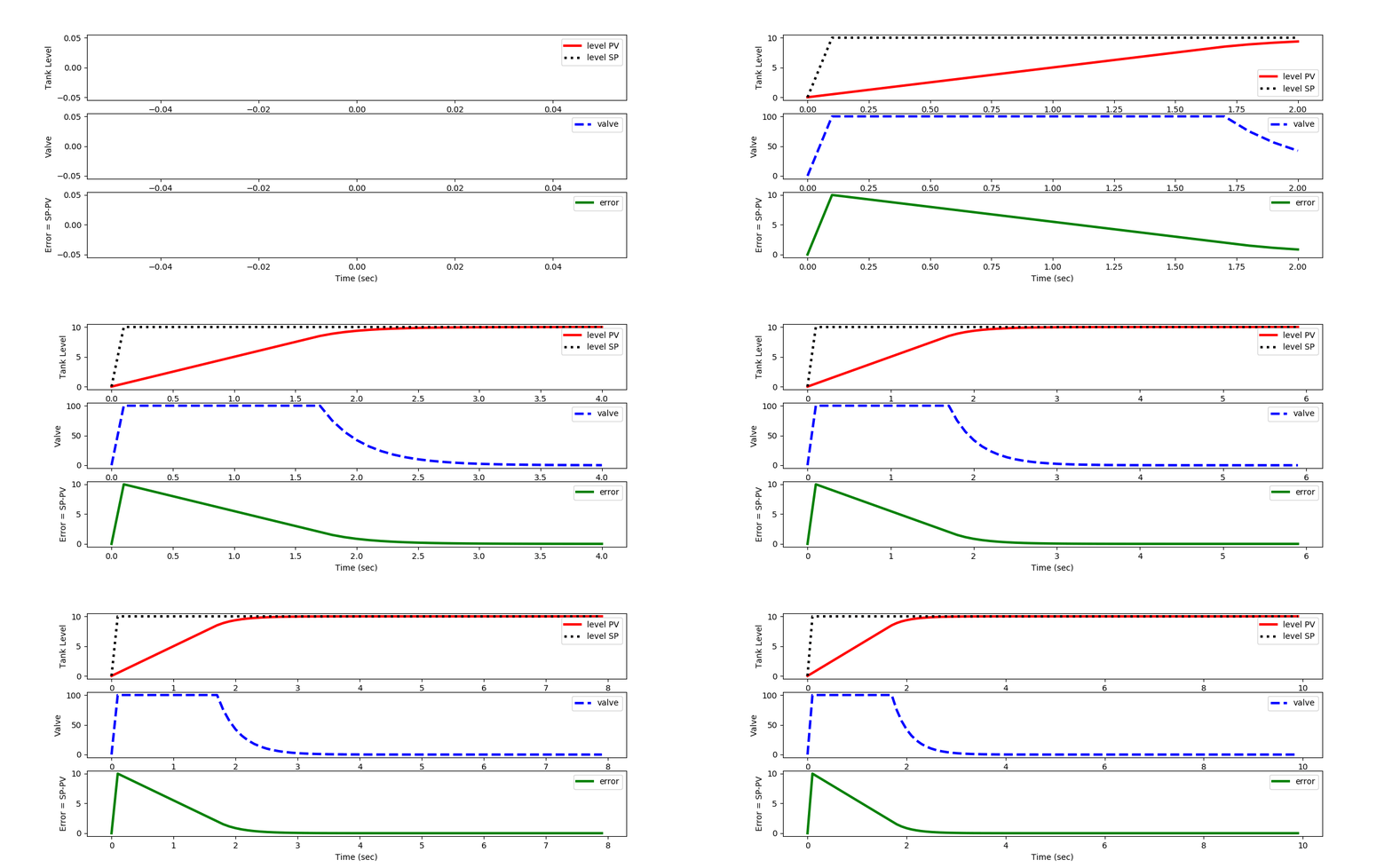
Design a P-only controller for the tank to maintain a level set point of 10.0 m. Test the P-only controller with different values of K_c by integrating the mass balance equation for a period of 10 seconds. Use a value of 1000 kg/m³ for density and 1.0 m² for the cross-sectional area of the tank. For the valve, assume a valve coefficient of c=50.0 (kg/s / percent open). Make sure that the valve does not exceed the limits of 0-100 percent by clipping the requested valve opening to an acceptable range. For example, if the P-only controller calculates a valve opening of 150 percent, use 100 percent instead.

Use the following Python script as a starting point for the simulation and add the Proportional-only controller. Select "Get Code" from the link at the bottom corner to get unformatted text. Fill in the areas labeled "TO DO" to implement the P-only controller.

Tank Level Control (Jupyter Notebook)

The IPython notebook source has two additional lines of code that animate the plot without creating a separate plot for each loop.

The following is the source code if not used in a notebook.

Solution

# solution
import numpy as np
import matplotlib.pyplot as plt
from scipy.integrate import odeint

# animate plots?
animate=True # True / False

# define tank model
def tank(Level,time,c,valve):
    rho = 1000.0 # water density (kg/m^3)
    A = 1.0      # tank area (m^2)
    # calculate derivative of the Level
    dLevel_dt = (c/(rho*A)) * valve
    return dLevel_dt

# time span for the simulation for 10 sec, every 0.1 sec
ts = np.linspace(0,10,101)

# valve operation
c = 50.0          # valve coefficient (kg/s / %open)
u = np.zeros(101) # u = valve % open

# level initial condition
Level0 = 0

# initial valve position
valve = 0

# for storing the results
z = np.zeros(101)
es = np.zeros(101)
sps = np.zeros(101)

# TO DO: what is the value for ubias?
ubias = 0

# TO DO: decide on a tuning value for Kc
Kc = 50.0

# TO DO: record the desired level (set point)
SP = 10

plt.figure(1,figsize=(12,5))
if animate:
    plt.ion()
    plt.show()
    make_gif = True
    try:
        import imageio  # required to make gif animation
    except:
        print('install imageio with "pip install imageio" to make gif')
        make_gif=False
    if make_gif:
        try:
            import os
            images = []
            os.mkdir('./frames')
        except:
            print('Figure directory failed')
            make_gif=False

# simulate with ODEINT
for i in range(100):
    # calculate the error
    error = SP - Level0

    # TO DO: put P-only controller here
    valve = ubias + Kc * error
    valve = max(0,valve)
    valve = min(100,valve)

    u[i+1] = valve   # store the valve position
    es[i+1] = error  # store the error
    y = odeint(tank,Level0,[0,0.1],args=(c,valve))
    Level0 = y[-1] # take the last point
    z[i+1] = Level0 # store the level for plotting
    sps[i+1] = SP

    if animate:
        # update plot
        plt.clf()
        plt.subplot(3,1,1)
        plt.plot(ts[0:i+1],z[0:i+1],'r-',linewidth=3,label='level PV')
        plt.plot(ts[0:i+1],sps[0:i+1],'k:',linewidth=3,label='level SP')
        plt.ylabel('Tank Level')
        plt.legend(loc='best')
        plt.subplot(3,1,2)
        plt.plot(ts[0:i+1],u[0:i+1],'b--',linewidth=3,label='valve')
        plt.ylabel('Valve')    
        plt.legend(loc='best')
        plt.subplot(3,1,3)
        plt.plot(ts[0:i+1],es[0:i+1],'g-',linewidth=3,label='error')
        plt.ylabel('Error = SP-PV')
        plt.xlabel('Time (sec)')
        plt.legend(loc='best')
        filename='./frames/frame_'+str(1000+i)+'.png'
        plt.savefig(filename)
        if make_gif:
            images.append(imageio.imread(filename))
        plt.pause(0.1)

if not animate:
    # plot results
    plt.subplot(3,1,1)
    plt.plot(ts,z,'r-',linewidth=3,label='level PV')
    plt.plot(ts,sps,'k:',linewidth=3,label='level SP')
    plt.ylabel('Tank Level')
    plt.legend(loc='best')
    plt.subplot(3,1,2)
    plt.plot(ts,u,'b--',linewidth=3,label='valve')
    plt.ylabel('Valve')    
    plt.legend(loc='best')
    plt.subplot(3,1,3)
    plt.plot(ts,es,'g-',linewidth=3,label='error')
    plt.ylabel('Error = SP-PV')    
    plt.xlabel('Time (sec)')
    plt.legend(loc='best')
    plt.show()
else:
    # create animated GIF
    if make_gif:
        imageio.mimsave('animate.gif', images)

[$[Get Code]]

---

Generative AI Learning

Use these prompts to test your understanding after completing the exercise. Direct the AI - do not let it do the exercise for you.

"Quiz me with 4 questions, one at a time, on level control with P-only action: why a gravity-drained tank is self-regulating while a pumped-outlet tank integrates, why P-only control leaves offset on the level and when that is acceptable in industry (surge tanks), how Kc changes the offset and the valve activity, and what happens at very high Kc with sensor noise. Grade my answers and list my misconceptions."

"My P-only level controller with Kc={value} settles at {level} for a setpoint of {setpoint}. Ask me to compute the expected offset from the process gain, compare with the measurement, and explain the difference. Then ask me whether I actually want zero offset on this tank, and challenge whichever answer I give with the surge-tank argument."

App: Run the experiment in the Tank Level Control Studio - fill the gravity-drained tank manually or with PID, add sensor noise and outlet-valve disturbances, and export the CSV; the animation makes the Bernoulli outflow visible.

What to Turn In

Submit a short report (PDF, 1-2 pages) that curates your results into a demonstration of what you learned. You may use Generative AI to help write the report, but you must guide it to the correct visualizations, justifications, and assumptions. Answer these questions:

1. Include level and valve plots for at least two Kc values (Python or app). Report the offset for each.
2. Is this tank self-regulating or integrating? Prove it with the model equation and one open-loop observation.
3. When is P-only control the RIGHT choice for a level loop? Give the surge-tank reasoning in your own words.
4. From the quiz prompt: one question you missed and the corrected answer.