Dynamic Optimization

(:html:) <iframe width="560" height="315" src="https://www.youtube.com/embed/daavzLUZqZY" frameborder="0" allow="accelerometer; autoplay; clipboard-write; encrypted-media; gyroscope; picture-in-picture" allowfullscreen></iframe> (:htmlend:)

See Introduction to Dynamic Estimation Examples 3 and 4 for IMODE=5 with differential equations and the Gekko IMODE Documentation.

• Linear Regression

See Introduction to Dynamic Estimation Examples 3 and 4 for IMODE=5 with differential equations and the Gekko IMODE Documentation.

<th class='text-small'>Mode (IMODE)</th>

<td class='text-left'><b>No Dynamics</b></td>

<td class='text-left'><b>Dynamic<br>Simultaneous</b></td>

<td class='text-left'><b>Dynamic<br>Sequential</b></td>

  height: 120px;

  width: 25%;

These examples do not have differential equations to describe dynamic systems. For problems with differential equations, use IMODE=5 instead of IMODE=2.

(:html:) <table class='table-fill'> <thead> <th class='text-small'></th> <th class='text-center'>Simulation</th> <th class='text-center'>Estimation</th> <th class='text-center'>Control</th> </thead>

<tbody class='table-hover'>

<tr> <td class='text-left'>Non-Dynamic</td> <td class='text-left'>1=Steady-State (SS)</td> <td class='text-left'>2=SS Regression (MPU)</td> <td class='text-left'>3=SS Optimize (RTO)</td> </tr>

<tr> <td class='text-left'>Dynamic Simultaneous</td> <td class='text-left'>4=Simulation (SIM)</td> <td class='text-left'>5=Estimation (EST)</td> <td class='text-left'>6=Control (CTL)</td> </tr>

<tr> <td class='text-left'>Dynamic Sequential</td> <td class='text-left'>7=Simulation (SQS)</td> <td class='text-left'>8=Estimation (EST)</td> <td class='text-left'>9=Control (CTL)</td> </tr>

</tbody> </table> (:htmlend:)

See Introduction to Dynamic Estimation Examples 3 and 4 for IMODE=5 with differential equations.

(:html:) <style type="text/css"> div.table-title {

   display: block;
  margin: auto;
  max-width: 600px;
  padding:5px;
  width: 100%;

}

.table-title h3 {

   color: #fafafa;

}

.table-fill {

  background: white;
  border-radius:3px;
  border-collapse: collapse;
  height: 320px;
  margin: auto;
  max-width: 600px;
  padding:5px;
  width: 100%;
  box-shadow: 0 5px 10px rgba(0, 0, 0, 0.1);
  animation: float 5s infinite;

}

th {

  color:#D5DDE5;;
  background:#1b1e24;
  border-bottom:4px solid #9ea7af;
  border-right: 1px solid #343a45;
  text-align:left;
  vertical-align:middle;

}

th:first-child {

  border-top-left-radius:3px;

}

th:last-child {

  border-top-right-radius:3px;
  border-right:none;

}

tr {

  border-top: 1px solid #C1C3D1;
  border-bottom-: 1px solid #C1C3D1;
  color:#666B85;
  font-weight:normal;

}

tr:hover td {

  border-top: 1px solid #22262e;
  border-bottom: 1px solid #22262e;

}

tr:first-child {

  border-top:none;

}

tr:last-child {

  border-bottom:none;

}

tr:nth-child(odd) td {

  background:#EEEEEE;

}

tr:last-child td:first-child {

  border-bottom-left-radius:3px;

}

tr:last-child td:last-child {

  border-bottom-right-radius:3px;

}

td {

  background:#FFFFFF;
  padding:5px;
  text-align:left;
  vertical-align:middle;
  border-right: 1px solid #C1C3D1;

}

td:last-child {

  border-right: 0px;

}

th.text-left {

  text-align: left;

}

th.text-center {

  text-align: center;

}

th.text-right {

  text-align: right;

}

td.text-left {

  text-align: left;
  width: 45%;

}

td.text-center {

  text-align: center;
  width: 10%;

}

td.text-small {

  text-align: center;
  width: 10%;

}

td.text-right {

  text-align: right;

} </style> (:htmlend:)

These examples do not have differential equations to describe dynamic systems. For problems with differential equations, use IMODE=5 instead of IMODE=2. See Introduction to Dynamic Estimation Examples 3 and 4 for IMODE=5 with differential equations.

Regression is used to train a model to predict a relationship between a dependent variable and one or more independent variables. Regression models can be linear or nonlinear, depending on the relationship between the dependent and independent variables. See the Machine Learning for Engineers course for additional information and the following tutorials:

• Linear Regression
• Nonlinear Regression
• Gaussian Processes
• k-Nearest Neighbors
• Linear Regression
• Neural Network Regressor
• Support Vector Regressor
• XGBoost Regressor

This tutorial is with linear regression to demonstrate a simple example in Python Gekko.

(:title Regression Introduction:) (:keywords regression, multiple, multivariate, tutorial:) (:description Multiple Linear Regression with Python Gekko with IMODE=2 and IMODE=3.:)

Regression is used to train a model to predict a relationship between a dependent variable and one or more independent variables. Regression models can be linear or nonlinear, depending on the relationship between the dependent and independent variables. See Linear Regression, Nonlinear Regression, and the Machine Learning for Engineers course for additional regression methods and examples. This tutorial is with linear regression to demonstrate a simple example in Python Gekko.

Example Multiple Linear Regression

Multiple linear regression models the relationship between a dependent variable and one or more independent variables. It is used when there are multiple independent variables that contribute to the prediction of the dependent variable. The goal of multiple linear regression is to find the best fit that minimizes the differences between the observed and predicted values of the dependent variable.

Objective: Perform multiple linear regression on sample data with two inputs.

Find unknown parameters c₀-c₂ to minimize the difference between measured ym and predicted yp subject to a constraint on the summation of c₁ x₁.

Data

$$x_1 = [1,2,5,3,2,5,2]$$

$$x_2 = [5,6,7,2,1,3,2]$$

$$y_m = [3,2,3,5,6,7,8]$$

Linear Equation

$$y_p = c_0 + c_1 x_1 + c_2 x_2$$

Constraint

$$0 \le \sum_{i=1}^n c_1 x_{1,i} \le 10$$

Minimize Objective

$$\min_{c} \sum_{i=1}^n \left(y_{m,i}-y_{p,i}\right)^2$$

where n is the length of y_m and c₀-c₂ are adjusted to minimize the sum of the squared errors. Report the parameter values and display a plot of the results.

Solution

Python Gekko has a regression mode where the equations are written once and applied over all data rows. The vsum object creates a vertical summation over a column.

(:toggle hide gekko2 button show="Show GEKKO IMODE=2 Solution":) (:div id=gekko2:)

(:source lang=python:) import numpy as np from gekko import GEKKO

1. load data

x1 = np.array([1,2,5,3,2,5,2]) x2 = np.array([5,6,7,2,1,3,2]) ym = np.array([3,2,3,5,6,7,8])

1. model

m = GEKKO() c = m.Array(m.FV,3) for ci in c:

    ci.STATUS=1

x1 = m.Param(value=x1) x2 = m.Param(value=x2) ymeas = m.Param(value=ym) ypred = m.Var() m.Equation(ypred == c[0] + c[1]*x1 + c[2]*x2)

1. add constraint on sum(c[1]*x1) with vsum

v1 = m.Var(); m.Equation(v1==c[1]*x1) con = m.Var(lb=0,ub=10); m.Equation(con==m.vsum(v1)) m.Minimize((ypred-ymeas)**2) m.options.IMODE = 2 m.solve() print('Final SSE Objective: ' + str(m.options.objfcnval)) print('Solution') for i,ci in enumerate(c):

    print(i,ci.value[0])

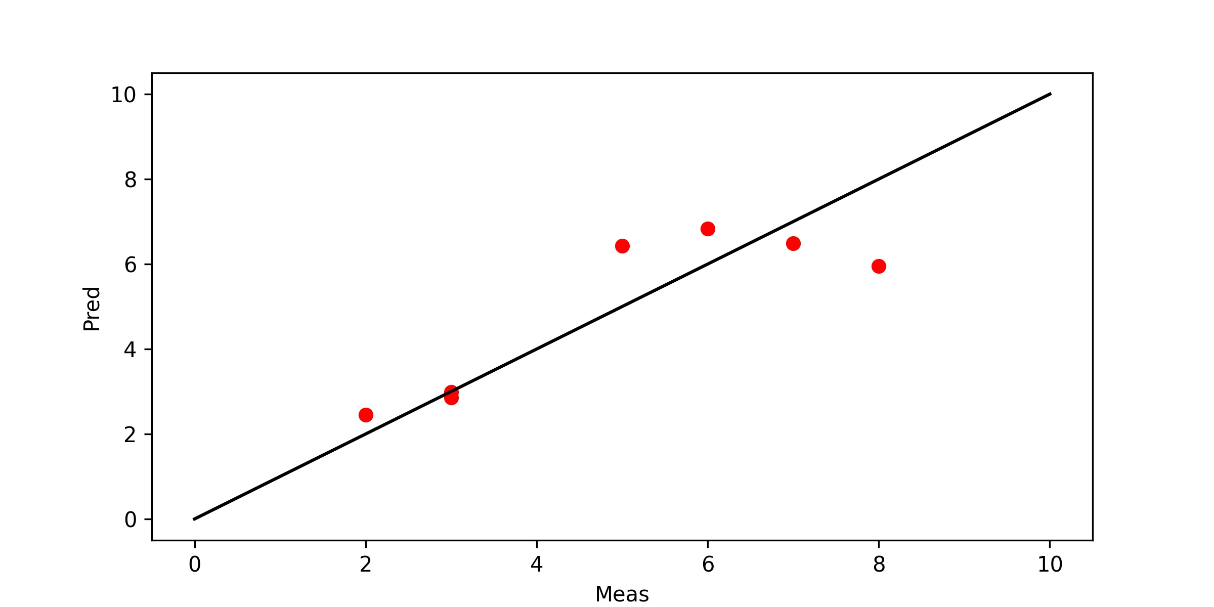
1. plot solution

import matplotlib.pyplot as plt plt.figure(figsize=(8,4)) plt.plot(ymeas,ypred,'ro') plt.plot([0,10],[0,10],'k-') plt.xlabel('Meas') plt.ylabel('Pred') plt.savefig('results.png',dpi=300) plt.show() (:sourceend:) (:divend:)

It is also possible to write each equation individually for additional control over the regression form. The IMODE=3 option is for optimization problems where each variable, objective term, and equation are written individually. IMODE=2 is more efficient for large-scale problems.

(:toggle hide gekko3 button show="Show GEKKO IMODE=3 Solution":) (:div id=gekko3:)

(:source lang=python:) import numpy as np from gekko import GEKKO

1. load data

x1 = np.array([1,2,5,3,2,5,2]) x2 = np.array([5,6,7,2,1,3,2]) ym = np.array([3,2,3,5,6,7,8]) n = len(ym)

1. model

m = GEKKO() c = m.Array(m.FV,3) for ci in c:

    ci.STATUS=1

yp = m.Array(m.Var,n) for i in range(n):

    m.Equation(yp[i]==c[0]+c[1]*x1[i]+c[2]*x2[i])
    m.Minimize((yp[i]-ym[i])**2)

1. add constraint on sum(c[1]*x1)

s = m.Var(lb=0,ub=10); m.Equation(s==c[1]*sum(x1)) m.options.IMODE = 3 m.solve() print('Final SSE Objective: ' + str(m.options.objfcnval)) print('Solution') for i,ci in enumerate(c):

    print(i,ci.value[0])

1. plot solution

import matplotlib.pyplot as plt plt.figure(figsize=(8,4)) ypv = [yp[i].value[0] for i in range(n)] plt.plot(ym,ypv,'ro') plt.plot([0,10],[0,10],'k-') plt.xlabel('Meas') plt.ylabel('Pred') plt.savefig('results.png',dpi=300) plt.show() (:sourceend:) (:divend:)

These examples do not have differential equations to describe dynamic systems. For problems with differential equations, use IMODE=5 instead of IMODE=2.