Solve Differential Equations
Main.ModelFormulation History
Show minor edits - Show changes to markup
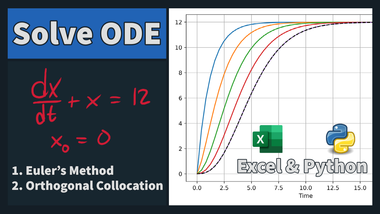 One of the most important factors in efficient and reliable solution of dynamic systems is the model formulation. Changes in model formulation are not intended to change the equations, only to put them into a form that allows solvers to more easily find an accurate solution. The ordinary differential equation `\frac{dx}{dt}+x=12` can be solved analytically with separate & integrate or LaPlace transforms. The ODE can also be solved numerically with Excel or Python. Differential equations can be solved with analytic or numerical methods. For numerical methods, one of the most important factors in efficient and reliable solution of dynamic systems is the model formulation. Changes in model formulation are not intended to change the equations, only to put them into a form that allows solvers to more easily find an accurate solution. The ordinary differential equation `\frac{dx}{dt}+x=12` can be solved analytically with separate & integrate or LaPlace transforms. The ODE can also be solved numerically with Excel or Python.
<iframe width="560" height="315" src="https://www.youtube.com/embed/CtUNKqynUak" title="YouTube video player" frameborder="0" allow="accelerometer; autoplay; clipboard-write; encrypted-media; gyroscope; picture-in-picture" allowfullscreen></iframe>
<iframe width="560" height="315" src="https://www.youtube.com/embed/7TbwDrZ3kAg" title="YouTube video player" frameborder="0" allow="accelerometer; autoplay; clipboard-write; encrypted-media; gyroscope; picture-in-picture" allowfullscreen></iframe>
(:title Formulation Strategies:)
(:title Solve Differential Equations:)
One of the most important factors in efficient and reliable solution of dynamic systems is the model formulation. Changes in model formulation are not intended to change the equations, only to put them into a form that allows solvers to more easily find an accurate solution. The ordinary differential equation `\frac{dx}{dt}+x=12` can be solved analytically with separate & integrate or LaPlace transforms. The ODE can also be solved numerically with Excel or Python. One of the most important factors in efficient and reliable solution of dynamic systems is the model formulation. Changes in model formulation are not intended to change the equations, only to put them into a form that allows solvers to more easily find an accurate solution. The ordinary differential equation `\frac{dx}{dt}+x=12` can be solved analytically with separate & integrate or LaPlace transforms. The ODE can also be solved numerically with Excel or Python. One of the most important factors in efficient and reliable solution of dynamic systems is the model formulation. Changes in model formulation are not intended to change the equations, only to put them into a form that allows solvers to more easily find an accurate solution. The ordinary differential equation `\frac{dx}{dt}+x=12` can be solved analytically with separate & integrate or LaPlace transforms. The ODE can also be solved numerically with Excel or Python. One of the most important factors in efficient and reliable solution of dynamic systems is the model formulation. Changes in model formulation are not intended to change the equations, only to put them into a form that allows solvers to more easily find an accurate solution. The ordinary differential equation `\frac{dx}{dt}+x=12` can be solved analytically with separate & integrate or LaPlace transforms. The ODE can also be solved numerically with Excel or Python. One of the most important factors in efficient and reliable solution of dynamic systems is the model formulation. Changes in model formulation are not intended to change the equations, only to put them into a form that allows solvers to more easily find an accurate solution. The ordinary differential equation `\frac{dx}{dt}+x=12` can be solved analytically with separate & integrate or LaPlace transforms. The ODE can also be solved numerically with Excel or Python. One of the most important factors in efficient and reliable solution of dynamic systems is the model formulation. Changes in model formulation are not intended to change the equations, only to put them into a form that allows solvers to more easily find an accurate solution. The ordinary differential equation `\frac{dx}{dt}+x=12` can be solved analytically with separate & integrate or LaPlace transforms. The ODE can also be solved numerically with Excel or Python.One of the most important factors in efficient and reliable solution of dynamic systems is the model formulation. Changes in model formulation are not intended to change the equations, only to put them into a form that allows solvers to more easily find an accurate solution. The ordinary differential equation `\frac{dx}{dt}+x=12` can be solved analytically with separate & integrate or LaPlace transforms. The ODE can also be solved numerically with Excel or Python.
One of the most important factors in efficient and reliable solution of dynamic systems is the model formulation. Changes in model formulation are not intended to change the equations, only to put them into a form that allows solvers to more easily find an accurate solution. The ordinary differential equation `\frac{dx}{dt}+x=12` can be solved analytically with separate & integrate or LaPlace transforms. The ODE can also be solved numerically with Excel or Python.One of the most important factors in efficient and reliable solution of dynamic systems is the model formulation. Changes in model formulation are not intended to change the equations, only to put them into a form that allows solvers to more easily find an accurate solution. The ordinary differential equation `\frac{dx}{dt}+x=12` can be solved analytically with separate & integrate or LaPlace transforms. It can also be solved numerically.
One of the most important factors in efficient and reliable solution of dynamic systems is the model formulation. Changes in model formulation are not intended to change the equations, only to put them into a form that allows solvers to more easily find an accurate solution. The ordinary differential equation `\frac{dx}{dt}+x=12` can be solved analytically with separate & integrate or LaPlace transforms. The ODE can also be solved numerically with Excel or Python.
(:html:) <iframe width="560" height="315" src="https://www.youtube.com/embed/CtUNKqynUak" title="YouTube video player" frameborder="0" allow="accelerometer; autoplay; clipboard-write; encrypted-media; gyroscope; picture-in-picture" allowfullscreen></iframe> (:htmlend:)
One of the most important factors in efficient and reliable solution of dynamic systems is the model formulation. Changes in model formulation are not intended to change the equations, only to put them into a form that allows solvers to more easily find an accurate solution. The ordinary differential equation `\frac{dx}{dt}+x=12` can be solved analytically with separate & integrate or LaPlace transforms. It can also be solved numerically with approximate methods.
One of the most important factors in efficient and reliable solution of dynamic systems is the model formulation. Changes in model formulation are not intended to change the equations, only to put them into a form that allows solvers to more easily find an accurate solution. The ordinary differential equation `\frac{dx}{dt}+x=12` can be solved analytically with separate & integrate or LaPlace transforms. It can also be solved numerically.
One of the most important factors in efficient and reliable solution of dynamic systems is the model formulation. Changes in model formulation are not intended to change the equations, only to put them into a form that allows solvers to more easily find an accurate solution. In each section below are some of the key strategies related to model creation and formulation. The discussion begins with a basic introduction to the APMonitor Modeling Language and Gekko Optimization Suite.
One of the most important factors in efficient and reliable solution of dynamic systems is the model formulation. Changes in model formulation are not intended to change the equations, only to put them into a form that allows solvers to more easily find an accurate solution. The ordinary differential equation `\frac{dx}{dt}+x=12` can be solved analytically with separate & integrate or LaPlace transforms. It can also be solved numerically with approximate methods.
(:source lang=python:) import numpy as np from gekko import GEKKO m = GEKKO(remote=False) m.time = np.linspace(0,5) x = m.Var(0) m.Equation(x.dt()+x==12) m.options.IMODE=4 m.solve(disp=False)
import matplotlib.pyplot as plt plt.plot(m.time,x) plt.show() (:sourceend:)
In each section below are some of the key strategies related to model creation and formulation. The discussion begins with a basic introduction to the APMonitor Modeling Language and Gekko Optimization Suite.
- Solve Differential Equations with Python Gekko
This course has examples in APM Matlab and Python Gekko. There are many other open-source simulation and optimization platforms that can also be used in this course.
(:source lang=python:) import numpy as np from gekko import GEKKO m = GEKKO(remote=False)
- input (1) = u
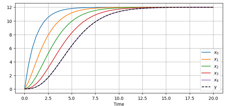
- states (5) = x[1] to x[5]
- output (1) = y
- Constants
n = 5 K = m.Const(4)
- Parameter
u = m.Param(value=3,lb=0,ub=10)
- Variable array
x = m.Array(m.Var,5,lb=0)
- Intermediate
y = m.Intermediate(x[4])
- Equations
m.Equation( x[0].dt() + x[0] == K*u) m.Equations([x[i].dt() + x[i] == x[i-1]
for i in range(1,n)])
- Objective
m.Minimize((y-5)**2)
- Define time
m.time = np.linspace(0,20)
- Solve dynamic simulation
m.options.IMODE = 4 m.solve()
- Show solution
import matplotlib.pyplot as plt for i in range(n):
plt.plot(m.time,x[i],label=f'$x_{i}$')
plt.plot(m.time,y,'k--',label='y') plt.xlabel('Time'); plt.grid(); plt.legend() plt.show() (:sourceend:)
This course has examples in APM Matlab and Python Gekko. See additional examples of solving differential equations in Python Gekko. There are many other open-source simulation and optimization platforms that can also be used in this course.
One of the most important factors in efficient and reliable solution of dynamic systems is the model formulation. Changes in model formulation are not intended to change the equations, only to put them into a form that allows solvers to more easily find an accurate solution. In each section below are some of the key strategies related to model creation and formulation. The discussion begins with a basic introduction to the APMonitor Modeling Language.
One of the most important factors in efficient and reliable solution of dynamic systems is the model formulation. Changes in model formulation are not intended to change the equations, only to put them into a form that allows solvers to more easily find an accurate solution. In each section below are some of the key strategies related to model creation and formulation. The discussion begins with a basic introduction to the APMonitor Modeling Language and Gekko Optimization Suite.
GEKKO is an object-oriented Python library to facilitate local execution of APMonitor. It is a Python package for machine learning and optimization of mixed-integer and differential algebraic equations. It is coupled with large-scale solvers for linear, quadratic, nonlinear, and mixed integer programming (LP, QP, NLP, MILP, MINLP). Modes of operation include parameter regression, data reconciliation, real-time optimization, dynamic simulation, and nonlinear predictive control.
GEKKO is an object-oriented Python library to facilitate local execution of APMonitor. It is a Python package for machine learning and optimization of mixed-integer and differential algebraic equations. It is coupled with large-scale solvers for linear, quadratic, nonlinear, and mixed integer programming (LP, QP, NLP, MILP, MINLP). Modes of operation include parameter regression, data reconciliation, real-time optimization, dynamic simulation, and nonlinear predictive control.
- Solve Differential Equations with Python Gekko
This course has examples in APM Matlab and Python Gekko. There are many other open-source simulation and optimization platforms that can also be used in this course.
APM MATLAB
 Reservoir Simulation in MATLAB with Video Solution
APM MATLAB
Reservoir Simulation in MATLAB with Video SolutionSlack variables are defined to transform an inequality expression into an equality expression with an added slack variable. The general expression for inequality constraints in the DAE expression is g(dx/dt,x,p)>0. An equivalent mathematical expression of the general inequality is g(dx/dt,x,p)=s and s>0. This form is desirable with solvers such as interior point methods where the initial guess must satisfy all inequality constraints or be on the inside of the feasible region. In the slack variable form, an initial guess value greater than zero for the new slack variable s satisfies this requirement. The APMonitor Modeling Language automatically transforms all inequality constraints into equivalent equality constraints with added slack variables.
- Click to Solve a Slack Variable Optimization Problem
(:html:) <iframe width="560" height="315" src="https://www.youtube.com/embed/jh6BK0BqqIs?rel=0" frameborder="0" allowfullscreen></iframe> (:htmlend:)
Slack variables are defined to transform an inequality expression into an equality expression with an added slack variable. The general expression for inequality constraints in the DAE expression is g(dx/dt,x,p)>0. An equivalent mathematical expression of the general inequality is g(dx/dt,x,p)=s and s>0. This form is desirable with solvers such as interior point methods where the initial guess must satisfy all inequality constraints or be on the inside of the feasible region. In the slack variable form, an initial guess value greater than zero for the new slack variable s satisfies this requirement. The APMonitor Modeling Language and Gekko Optimization Suite automatically transform all inequality constraints into equivalent equality constraints with added slack variables. See additional information (video) on slack variables.
(:html:) <iframe width="560" height="315" src="https://www.youtube.com/embed/ZzYURrtD4YI?rel=0" frameborder="0" allowfullscreen></iframe>(:htmlend:)
APMonitor Modeling Language
Gekko Optimization Suite
GEKKO is an object-oriented Python library to facilitate local execution of APMonitor. It is a Python package for machine learning and optimization of mixed-integer and differential algebraic equations. It is coupled with large-scale solvers for linear, quadratic, nonlinear, and mixed integer programming (LP, QP, NLP, MILP, MINLP). Modes of operation include parameter regression, data reconciliation, real-time optimization, dynamic simulation, and nonlinear predictive control.
There is an additional optional designation of parameters as either fixed values (FVs) or manipulated variables (MVs). Variables can be optionally designated as state variables (SVs) or controlled variables (CVs). The terminology of FV, MV, SV, and CV is from the process systems engineering community. In this community the MVs are designated as the inputs that are potentially changed by the controller and CVs are model outputs that are driven to target conditions. The terms FVs refer to either measured or unmeasured disturbances to the system and SVs are simply designated for viewing purposes as variables of importance. These parameter and variable classifications are specified in MATLAB or Python scripts (See additional details on FV, MV, SV, and CV classification).
There is an additional optional designation of parameters as either fixed values (FVs) or manipulated variables (MVs). Variables can be optionally designated as state variables (SVs) or controlled variables (CVs). The terminology of FV, MV, SV, and CV is from the process systems engineering community. In this community the MVs are designated as the inputs that are potentially changed by the operator or controller as external decisions that are degrees of freedom to minimize an objective function. The CVs are model outputs that are defined by equations and driven to target conditions. The terms FVs refer to either measured or unmeasured disturbances to the system. SVs are simply designated for viewing purposes as variables of importance. These parameter and variable classifications are specified in MATLAB or Python scripts (See additional details on FV, MV, SV, and CV classification).
Vflow_in1 = 0.13 (July-Mar), 0.21 (Apr-June)
Vflow_in1 = 0.13 (June-Feb), 0.21 (Mar-May)
vin = [0.13,0.13,0.13,0.13,0.21,0.21,0.21,\
vin = [0.13,0.13,0.13,0.21,0.21,0.21,0.13,\
vin = [0.13,0.13,0.13,0.21,0.21,0.21,0.13,\
vin = [0.13,0.13,0.13,0.13,0.21,0.21,0.21,\
Outflow River Rates (km3/yr)
Outflow River Rates (km3/yr) with height in meters
(:html:) <iframe width="560" height="315" src="https://www.youtube.com/embed/BHxNe86_TXc" frameborder="0" gesture="media" allow="encrypted-media" allowfullscreen></iframe> (:htmlend:)
(:toggle hide gekko button show="Show GEKKO (Python) Code":) (:div id=gekko:) (:source lang=python:) from __future__ import division from gekko import GEKKO import numpy as np
- Initial conditions
c = np.array([0.03,0.015,0.06,0]) areas = np.array([13.4, 12, 384.5, 4400]) V0 = np.array([0.26, 0.18, 0.68, 22]) h0 = 1000 * V0 / areas Vout0 = c * np.sqrt(h0) vin = [0.13,0.13,0.13,0.21,0.21,0.21,0.13, 0.13,0.13,0.13,0.13,0.13,0.13] Vin = [0,0,0,0]
- Initialize model
m = GEKKO()
- time array
m.time = np.linspace(0,1,13)
- define constants
c = m.Array(m.Const,4,value=0) c[0].value = 0.03 c[1].value = c[0] / 2 c[2].value = c[0] * 2 c[3].value = 0 Vuse = [0.03,0.05,0.02,0.00]
- Parameters
evap_c = m.Array(m.Param,4,value=1e-5) evap_c[-1].value = 0.5e-5
A = [m.Param(value=i) for i in areas]
Vin[0] = m.Param(value=vin)
- Variables
V = [m.Var(value=i) for i in V0] h = [m.Var(value=i) for i in h0] Vout = [m.Var(value=i) for i in Vout0]
- Intermediates
Vin[1:4] = [m.Intermediate(Vout[i]) for i in range(3)] Vevap = [m.Intermediate(evap_c[i] * A[i]) for i in range(4)]
- Equations
m.Equations([V[i].dt() == Vin[i] - Vout[i] - Vevap[i] - Vuse[i] for i in range(4)]) m.Equations([1000*V[i] == h[i]*A[i] for i in range(4)]) m.Equations([Vout[i]**2 == c[i]**2 * h[i] for i in range(4)])
- Set to simulation mode
m.options.imode = 4
- Solve
m.solve()
- Plot results
time = [x * 12 for x in m.time]
- plot results
import matplotlib.pyplot as plt plt.figure(1)
plt.subplot(311) plt.plot(time,h[0].value,'r-') plt.plot(time,h[1].value,'b--') plt.ylabel('Level (m)') plt.legend(['Jordanelle Reservoir','Deer Creek Reservoir'])
plt.subplot(312) plt.plot(time,h[3].value,'g-') plt.plot(time,h[2].value,'k:') plt.ylabel('Level (m)') plt.legend(['Great Salt Lake','Utah Lake'])
plt.subplot(313) plt.plot(time,Vin[0].value,'k-') plt.plot(time,Vout[0].value,'r-') plt.plot(time,Vout[1].value,'b--') plt.plot(time,Vout[2].value,'g-') plt.xlabel('Time (month)') plt.ylabel('Flow (km3/yr)') plt.legend(['Supply Flow','Upper Provo River', 'Lower Provo River','Jordan River']) plt.show() (:sourceend:) (:divend:)
 Vevap1 = 0.03
 Vevap2 = 0.05
 Vevap3 = 0.02
 Vevap4 = 0.00
 Vuse1 = 0.03
 Vuse2 = 0.05
 Vuse3 = 0.02
 Vuse4 = 0.00
Simulate the height of the reservoirs over the course of a year, starting in January, with higher inlet flowrates in the spring due to melting snow. Use a mass balance to describe the change in volume and height of each body of water. This is a simple simulation model that assumes no active control. In actual practice, water outlet flows are actively managed to maintain reservoir levels for recreation, provide sufficient river flow rates, limit river flow rates to avoid flooding, and serve agricultural and community needs. Utah Lake and the Great Salt Lake also have additional inlet sources such as the Payson River (Utah Lake) and the Weber River and Bear River (Great Salt Lake) that are not considered in this simulation.
Simulate the height of the reservoirs (in meters) over the course of a year, starting in January, with higher inlet flowrates in the spring due to melting snow. Use a mass balance to describe the change in volume and height of each body of water. This is a simple simulation model that assumes no active control. In actual practice, water outlet flows are actively managed to maintain reservoir levels for recreation, provide sufficient river flow rates, limit river flow rates to avoid flooding, and serve agricultural and community needs. Utah Lake and the Great Salt Lake also have additional inlet sources such as the Payson River (Utah Lake) and the Weber River and Bear River (Great Salt Lake) that are not considered in this simulation.
Simulate the height of the reservoirs over the course of a year, starting in January, with higher inlet flowrates in the spring due to melting snow. This is a simple simulation model that assumes no active control. In actual practice, water outlet flows are actively managed to maintain reservoir levels for recreation, provide sufficient river flow rates, limit river flow rates to avoid flooding, and serve agricultural and community needs. Utah Lake and the Great Salt Lake also have additional inlet sources such as the Payson River (Utah Lake) and the Weber River and Bear River (Great Salt Lake) that are not considered in this simulation.
Simulate the height of the reservoirs over the course of a year, starting in January, with higher inlet flowrates in the spring due to melting snow. Use a mass balance to describe the change in volume and height of each body of water. This is a simple simulation model that assumes no active control. In actual practice, water outlet flows are actively managed to maintain reservoir levels for recreation, provide sufficient river flow rates, limit river flow rates to avoid flooding, and serve agricultural and community needs. Utah Lake and the Great Salt Lake also have additional inlet sources such as the Payson River (Utah Lake) and the Weber River and Bear River (Great Salt Lake) that are not considered in this simulation.
<iframe width="560" height="315" src="https://www.youtube.com/embed/WCTTY4baYLk?rel=0" frameborder="0" allowfullscreen></iframe> (:htmlend:)
<iframe width="560" height="315" src="https://www.youtube.com/embed/ZzYURrtD4YI?rel=0" frameborder="0" allowfullscreen></iframe>(:htmlend:)
Objective: Formulate a dynamic model with model quantities such as constants, parameters, and variables and model expressions such as intermediates and equations. Use time-varying inputs, initial conditions, and mass balance equations to specify the problem inputs and dynamics. Create a MATLAB or Python script to simulate and display the results.
Objective: Formulate a dynamic model with model quantities such as constants, parameters, and variables and model expressions such as intermediates and equations. Use time-varying inputs, initial conditions, and mass balance equations to specify the problem inputs and dynamics. Create a MATLAB or Python script to simulate and display the results. Estimated Time: 2 hours
Objective: Formulate a dynamic model with model quantities such as constants, parameters, and variables and model expressions such as intermediates and equations. Use time-varying inputs, initial conditions, and mass balance equations to specify the problem inputs and dynamics. Create a MATLAB or Python script to simulate and display the results.
Simulate the height of the reservoirs over the course of a year, starting in January, with higher inlet flowrates in the spring due to melting snow. This is a simple simulation model that assumes no active control. In actual practice, water outlet flows are actively managed to maintain reservoir levels for recreation, provide sufficient river flow rates, limit river flow rates to avoid flooding, and serve agricultural and community needs.
Simulate the height of the reservoirs over the course of a year, starting in January, with higher inlet flowrates in the spring due to melting snow. This is a simple simulation model that assumes no active control. In actual practice, water outlet flows are actively managed to maintain reservoir levels for recreation, provide sufficient river flow rates, limit river flow rates to avoid flooding, and serve agricultural and community needs. Utah Lake and the Great Salt Lake also have additional inlet sources such as the Payson River (Utah Lake) and the Weber River and Bear River (Great Salt Lake) that are not considered in this simulation.
 Area of Reservoir / Lake (km2)
 A1 = 13.4
 A2 = 12.0
 A3 = 384.5
 A4 = 4400
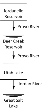
Suppose that there is a spillway from each upstream body of water to the lower body of water with a flow that is proportional to the square root of the reservoir height. There is no outflow from the Great Salt Lake except due to evaporation. Develop a simplified dynamic model of the height change in each reservoir from water mass balances. Below are relevant constants to use for outflow correlations and initial holdups. Below are constants such as area (km2) and usage requirements (km3/yr), inlet and outlet flow correlations (km3/yr), and initial conditions for the volumes (km3).
Suppose that there is a spillway from each upstream body of water to the lower body of water with a flow that is proportional to the square root of the reservoir height. There is no outflow from the Great Salt Lake except due to evaporation. Develop a simplified dynamic model of the height change in each reservoir from water mass balances. Below are constants such as area (km2) and usage requirements (km3/yr), inlet and outlet flow correlations (km3/yr), evaporation correlations, and initial conditions for the volumes (km3).
(:table border=0 width=100%:) (:cell width=20%:)
(:cell width=80%:)
(:tableend:)
(:html:) <iframe width="560" height="315" src="https://www.youtube.com/embed/WCTTY4baYLk?rel=0" frameborder="0" allowfullscreen></iframe> (:htmlend:)
 V'_evap' = 1e-5 * Area, for fresh water
 V'_evap' = 0.5e-5 * Area, for salt water
 Vevap = 0.5e-5 * Area, for salt water (Great Salt Lake)
 Vevap = 1e-5 * Area, for fresh water (all others)
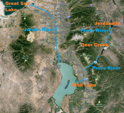
In Utah, water flows into the (1) Jordanelle reservoir, to the (2) Deer Creek reservoir, to (3) Utah Lake, and finally to the (4) Great Salt Lake. Suppose that there is a spillway from each upstream body of water to the lower body of water with a flow that is proportional to the square root of the reservoir height. There is no outflow from the Great Salt Lake except due to evaporation. Develop a simplified dynamic model of the height change in each reservoir from water mass balances. Below are relevant constants to use for outflow correlations and initial holdups. Below are constants such as area (km2) and usage requirements (km3/yr), inlet and outlet flow correlations (km3/yr), and initial conditions for the volumes (km3).
 Outflow Rates (km3/yr)
 Vflow_out1 = 0.1 sqrt(h1)
 Vflow_out2 = 0.05 sqrt(h2)
 Vflow_out3 = 0.2 sqrt(h3)
In Utah, water flows into the (1) Jordanelle reservoir, to the (2) Deer Creek reservoir, to (3) Utah Lake, and finally to the (4) Great Salt Lake.
Suppose that there is a spillway from each upstream body of water to the lower body of water with a flow that is proportional to the square root of the reservoir height. There is no outflow from the Great Salt Lake except due to evaporation. Develop a simplified dynamic model of the height change in each reservoir from water mass balances. Below are relevant constants to use for outflow correlations and initial holdups. Below are constants such as area (km2) and usage requirements (km3/yr), inlet and outlet flow correlations (km3/yr), and initial conditions for the volumes (km3).
 Outflow River Rates (km3/yr)
 Vflow_out1 = 0.030 sqrt(h1)
 Vflow_out2 = 0.015 sqrt(h2)
 Vflow_out3 = 0.060 sqrt(h3)
 Evaporation Rates (km3/yr)
 V'_evap' = 1e-5 * Area, for fresh water
 V'_evap' = 0.5e-5 * Area, for salt water
 Evaporation Rates (km3/yr)
 Vevap1 = 0.01 A1
 Vevap2 = 0.01 A2
 Vevap3 = 0.01 A3
 Vevap4 = 0.005 A4
 Vevap1 = 20
 Vevap2 = 100
 Vevap3 = 30
 Vevap4 = 0
 Vevap1 = 0.03
 Vevap2 = 0.05
 Vevap3 = 0.02
 Vevap4 = 0.00

 Area of Reservoir / Lake (km2)
 A1 = 13.4
 A2 = 12.0
 A3 = 384.5
 A4 = 4400

 Area of Reservoir / Lake (km2)
 A1 = 13.4
 A2 = 12.0
 A3 = 384.5
 A4 = 4400

 Initial Volume of Reservoir / Lake (km3)
 V1 = 0.26
 V2 = 0.18
 V3 = 0.68
 V4 = 22.0
In Utah, water flows into the (1) Jordanelle reservoir, to the (2) Deer Creek reservoir, to (3) Utah Lake, and finally to the (4) Great Salt Lake. Suppose that there is a spillway from each upstream body of water to the lower body of water with a flow that is proportional to the square root of the reservoir height. There is no outflow from the Great Salt Lake except due to evaporation. Develop a simplified dynamic model of the height change in each reservoir from water mass balances. Below are relevant constants to use for outflow correlations and initial holdups. Lookup estimates for the height (km), area (km2), and initial volumes (km3). Simulate the height of the reservoirs over the course of a year with higher inlet flowrates in the spring due to melting snow.
 Vflow_in1 = variable
 Vflow_in2 = Vflow_out1
 Vflow_in3 = Vflow_out2
 Vflow_in4 = Vflow_out3
In Utah, water flows into the (1) Jordanelle reservoir, to the (2) Deer Creek reservoir, to (3) Utah Lake, and finally to the (4) Great Salt Lake. Suppose that there is a spillway from each upstream body of water to the lower body of water with a flow that is proportional to the square root of the reservoir height. There is no outflow from the Great Salt Lake except due to evaporation. Develop a simplified dynamic model of the height change in each reservoir from water mass balances. Below are relevant constants to use for outflow correlations and initial holdups. Below are constants such as area (km2) and usage requirements (km3/yr), inlet and outlet flow correlations (km3/yr), and initial conditions for the volumes (km3).
Outflow Rates (km3/yr)
 Inflow Rates (km3/yr)
 Vflow_in1 = 0.13 (July-Mar), 0.21 (Apr-June)
 Vflow_in2 = Vflow_out1
 Vflow_in3 = Vflow_out2
 Vflow_in4 = Vflow_out3

 Evaporation Rates (km3/yr)
 Usage Requirements (km3/yr)
 Vevap1 = 20
 Vevap2 = 100
 Vevap3 = 30
 Vevap4 = 0
This is a simple simulation model that assumes no active control. In actual practice, water outlet flows are actively managed to maintain reservoir levels for recreation, provide sufficient river flow rates, limit river flow rates to avoid flooding, and serve agricultural and community needs.
Simulate the height of the reservoirs over the course of a year, starting in January, with higher inlet flowrates in the spring due to melting snow. This is a simple simulation model that assumes no active control. In actual practice, water outlet flows are actively managed to maintain reservoir levels for recreation, provide sufficient river flow rates, limit river flow rates to avoid flooding, and serve agricultural and community needs.
In Utah, water flows into the (1) Jordanelle reservoir, to the (2) Deer Creek reservoir, to (3) Utah Lake, and finally to the (4) Great Salt Lake. Suppose that there is a spillway from each upstream body of water to the lower body of water with a flow that is proportional to the square root of the reservoir height. There is no outflow from the Great Salt Lake except due to evaporation. Develop a simplified dynamic model of the height change in each reservoir from water mass balances. Below are relevant constants to use for outflow correlations and initial holdups. Lookup estimates for the height (m), area (m2), and initial volumes (m3). Simulate the height of the reservoirs over the course of a year with higher inlet flowrates in the spring due to melting snow.
In Utah, water flows into the (1) Jordanelle reservoir, to the (2) Deer Creek reservoir, to (3) Utah Lake, and finally to the (4) Great Salt Lake. Suppose that there is a spillway from each upstream body of water to the lower body of water with a flow that is proportional to the square root of the reservoir height. There is no outflow from the Great Salt Lake except due to evaporation. Develop a simplified dynamic model of the height change in each reservoir from water mass balances. Below are relevant constants to use for outflow correlations and initial holdups. Lookup estimates for the height (km), area (km2), and initial volumes (km3). Simulate the height of the reservoirs over the course of a year with higher inlet flowrates in the spring due to melting snow.
 Vflow_in2 = mout1
 V'flow_in3' = mout2
 V'flow_in4' = mout3
 Vflow_out1 = 0.1 sqrt(h1)
 Vflow_out2 = 0.05 sqrt(h2)
 Vflow_out3 = 0.2 sqrt(h3)
 Vflow_out4 = 0
 Vevap1 = 0.01 A1
 Vevap2 = 0.01 A2
 Vevap3 = 0.01 A3
 Vevap3 = 0.005 A4
 Vflow_in2 = Vflow_out1
 Vflow_in3 = Vflow_out2
 Vflow_in4 = Vflow_out3
 Vflow_out1 = 0.1 sqrt(h1)
 Vflow_out2 = 0.05 sqrt(h2)
 Vflow_out3 = 0.2 sqrt(h3)
 Vflow_out4 = 0
 Vevap1 = 0.01 A1
 Vevap2 = 0.01 A2
 Vevap3 = 0.01 A3
 Vevap3 = 0.005 A4
 V'flow_in1' = variable
 V'flow_in2' = m'_out1'
 V'flow_in3' = m'_out2'
 V'flow_in4' = m'_out3'
 Vflow_in1 = variable
 Vflow_in2 = mout1
 V'flow_in3' = mout2
 V'flow_in4' = mout3
In Utah, water flows into the (1) Jordanelle reservoir, to the (2) Deer Creek reservoir, to (3) Utah Lake, and finally to the (4) Great Salt Lake. Suppose that there is a spillway from each upstream body of water to the lower body of water with a flow that is proportional to the square root of the reservoir height. There is no outflow from the Great Salt Lake except due to evaporation. Develop a simplified dynamic model of the height change in each reservoir from water mass balances. Below are relevant constants to use for outflow correlations and initial holdups. Lookup estimates for the height (m) and area (m^_2_^).
 m^_out1^ = 0.1 h^_1_^
 m^_out2^ = 0.05 h^_2_^
 m^_out3^ = 0.2 h^_3_^
 m^_out4^ = 0
 m^_evap1^ = 0.01 A^_1_^
 m^_evap2^ = 0.01 A^_2_^
 m^_evap3^ = 0.01 A^_3_^
 m^_evap3^ = 0.005 A^_4_^
In Utah, water flows into the (1) Jordanelle reservoir, to the (2) Deer Creek reservoir, to (3) Utah Lake, and finally to the (4) Great Salt Lake. Suppose that there is a spillway from each upstream body of water to the lower body of water with a flow that is proportional to the square root of the reservoir height. There is no outflow from the Great Salt Lake except due to evaporation. Develop a simplified dynamic model of the height change in each reservoir from water mass balances. Below are relevant constants to use for outflow correlations and initial holdups. Lookup estimates for the height (m), area (m2), and initial volumes (m3). Simulate the height of the reservoirs over the course of a year with higher inlet flowrates in the spring due to melting snow.
 V'flow_in1' = variable
 V'flow_in2' = m'_out1'
 V'flow_in3' = m'_out2'
 V'flow_in4' = m'_out3'
 Vflow_out1 = 0.1 sqrt(h1)
 Vflow_out2 = 0.05 sqrt(h2)
 Vflow_out3 = 0.2 sqrt(h3)
 Vflow_out4 = 0
 Vevap1 = 0.01 A1
 Vevap2 = 0.01 A2
 Vevap3 = 0.01 A3
 Vevap3 = 0.005 A4
Solution
In Utah, water flows into the (1) Jordanelle reservoir, to the (2) Deer Creek reservoir, to (3) Utah Lake, and finally to the (4) Great Salt Lake. Suppose that there is a spillway from each upstream body of water to the lower body of water with a flow that is proportional to the square root of the reservoir height. There is no outflow from the Great Salt Lake except due to evaporation. Develop a simplified dynamic model of the height change in each reservoir from water mass balances. Below are relevant constants to use for outflow correlations and initial holdups. Lookup estimates for the height (m) and area (m^_2_^).
 m^_out1^ = 0.1 h^_1_^
 m^_out2^ = 0.05 h^_2_^
 m^_out3^ = 0.2 h^_3_^
 m^_out4^ = 0
 m^_evap1^ = 0.01 A^_1_^
 m^_evap2^ = 0.01 A^_2_^
 m^_evap3^ = 0.01 A^_3_^
 m^_evap3^ = 0.005 A^_4_^
This is a simple simulation model that assumes no active control. In actual practice, water outlet flows are actively managed to maintain reservoir levels for recreation, provide sufficient river flow rates, limit river flow rates to avoid flooding, and serve agricultural and community needs.
Solution
Slack variables are defined to transform an inequality expression into an equality expression with an added slack variable. The general expression for inequality constraints in the DAE expression is g(dx/dt,x,p)>0. An equivalent mathematical expression of the general inequality is g(dx/dt,x,p)=s and s>0. This form is desirable with solvers such as interior point methods where the initial guess must satisfy all inequality constraints or be on the inside of the feasible region. In the slack variable form, an initial guess value greater than zero for the new slack variable s satisfies this requirement. The APMonitor Modeling Language automatically transforms all inequality constraints into equivalent equality constraints with added slack variables.
Slack variables are defined to transform an inequality expression into an equality expression with an added slack variable. The general expression for inequality constraints in the DAE expression is g(dx/dt,x,p)>0. An equivalent mathematical expression of the general inequality is g(dx/dt,x,p)=s and s>0. This form is desirable with solvers such as interior point methods where the initial guess must satisfy all inequality constraints or be on the inside of the feasible region. In the slack variable form, an initial guess value greater than zero for the new slack variable s satisfies this requirement. The APMonitor Modeling Language automatically transforms all inequality constraints into equivalent equality constraints with added slack variables.
(:html:) <iframe width="560" height="315" src="https://www.youtube.com/embed/ELEUFKzwUj0" frameborder="0" allowfullscreen></iframe> (:htmlend:)
- Click to Solve a Slack Variable Optimization Problem
(:html:) <iframe width="560" height="315" src="https://www.youtube.com/embed/jh6BK0BqqIs?rel=0" frameborder="0" allowfullscreen></iframe> (:html:)
There is an additional optional designation of parameters as either fixed values (FVs) or manipulated variables (MVs). Variables can be optionally designated as state variables (SVs) or controlled variables (CVs). The terminology of FV, MV, SV, and CV is from the process systems engineering community. In this community the MVs are designated as the inputs that are potentially changed by the controller and CVs are model outputs that are driven to target conditions. The terms FVs refer to either measured or unmeasured disturbances to the system and SVs are simply designated for viewing purposes as variables of importance. These parameter and variable classifications are specified in MATLAB or Python scripts (See additional details on FV, MV, SV, and CV classification).
Collections of constants, parameters, variables, intermediates, equations, objects, and connections constitute a model. The model file is created and stored in a text file with extension apm. Several text editors are available that support syntax highlighting such as Notepad++ and gEdit (---see installation instructions). Below is an example model that demonstrates the use of many of these sections to create a 5th order differential equation model.
There is an additional optional designation of parameters as either fixed values (FVs) or manipulated variables (MVs). Variables can be optionally designated as state variables (SVs) or controlled variables (CVs). The terminology of FV, MV, SV, and CV is from the process systems engineering community. In this community the MVs are designated as the inputs that are potentially changed by the controller and CVs are model outputs that are driven to target conditions. The terms FVs refer to either measured or unmeasured disturbances to the system and SVs are simply designated for viewing purposes as variables of importance. These parameter and variable classifications are specified in MATLAB or Python scripts (See additional details on FV, MV, SV, and CV classification).
Collections of constants, parameters, variables, intermediates, equations, objects, and connections constitute a model. The model file is created and stored in a text file with extension apm. Several text editors are available that support syntax highlighting such as Notepad++ and gEdit (see installation instructions). Below is an example model that demonstrates the use of many of these sections to create a 5th order differential equation model.
Certain functions such as abs, if..then, min, max, signum, and discontinuous functions can be included in models but need to be posed in a way to allow efficient solution by solvers that perform better with continuous first and second derivatives. There are alternative methods to reformulate the problems. Two popular approaches are as MPECs (Mathematical Programs with Equilibrium Constraints) or with binary variables that switch on or off certain elements of the equations.
Certain functions such as abs, if..then, min, max, signum, and discontinuous functions can be included in models but need to be posed in a way to allow efficient solution by solvers that perform better with continuous first and second derivatives. There are alternative methods to reformulate the problems. Two popular approaches are as MPECs (Mathematical Programs with Equilibrium Constraints) or with binary variables that switch on or off certain elements of the equations.
There is an additional optional designation of parameters as either fixed values (FVs) or manipulated variables (MVs). Variables can be optionally designated as state variables (SVs) or controlled variables (CVs). The terminology of FV, MV, SV, and CV is from the process systems engineering community. In this community the MVs are designated as the inputs that are potentially changed by the controller and CVs are model outputs that are driven to target conditions. The terms FVs refer to either measured or unmeasured disturbances to the system and SVs are simply designated for viewing purposes as variables of importance. These parameter and variable classifications are specified in MATLAB or Python scripts.
There is an additional optional designation of parameters as either fixed values (FVs) or manipulated variables (MVs). Variables can be optionally designated as state variables (SVs) or controlled variables (CVs). The terminology of FV, MV, SV, and CV is from the process systems engineering community. In this community the MVs are designated as the inputs that are potentially changed by the controller and CVs are model outputs that are driven to target conditions. The terms FVs refer to either measured or unmeasured disturbances to the system and SVs are simply designated for viewing purposes as variables of importance. These parameter and variable classifications are specified in MATLAB or Python scripts (See additional details on FV, MV, SV, and CV classification).
(--include link to additional symbols--)
MPECs - max, min, abs, if statements, etc
Certain functions such as abs, if..then, min, max, signum, and discontinuous functions can be included in models but need to be posed in a way to allow efficient solution by solvers that perform better with continuous first and second derivatives. There are alternative methods to reformulate the problems. Two popular approaches are as MPECs (Mathematical Programs with Equilibrium Constraints) or with binary variables that switch on or off certain elements of the equations.
- Equations are either equality constraints as f(dx/dt,x,p)=0, inequality constraints as g(dx/dt,x,p)>0, or expression of the objective with statements that begin with keywords maximize or minimize.
- Equations are either equality constraints as f(dx/dt,x,p)=0, inequality constraints as g(dx/dt,x,p)>0, or expression of the objective with statements that begin with keywords maximize or minimize (See additional details on equations).
- Constants are values that never change. Integer values may be defined to give sizes to arrays (See additional details on constants)..
- Constants are values that never change. Integer values may be defined to give sizes to arrays (See additional details on constants).
- Constants are values that never change. Integer values may be defined to give sizes to arrays.
- Parameters are values that are nominally fixed at initial values but can be changed with input data, by the user, or can become calculated by the optimizer to minimize an objective function if they are indicated as decision variables.
- Variables are always calculated values as determined by the set of equations. Some variables are either measured and/or controlled to a desired target value.
- Intermediates are explicit equations where the variable is set equal to an expression that may include constants, parameters, variables, or other intermediate values that are defined previously. Intermediates are not implicit equations but are explicitly calculated with each model function evaluation.
- Constants are values that never change. Integer values may be defined to give sizes to arrays (See additional details on constants)..
- Parameters are values that are nominally fixed at initial values but can be changed with input data, by the user, or can become calculated by the optimizer to minimize an objective function if they are indicated as decision variables (See additional details on parameters).
- Variables are always calculated values as determined by the set of equations. Some variables are either measured and/or controlled to a desired target value (See additional details on variables).
- Intermediates are explicit equations where the variable is set equal to an expression that may include constants, parameters, variables, or other intermediate values that are defined previously. Intermediates are not implicit equations but are explicitly calculated with each model function evaluation (See additional details on intermediates).
- Objects are object-oriented extensions of APMonitor that may include parameters, variables, equations, and objective terms.
- Connections are simple equality constraints that relate object variables to model parameter or variables.
There is an additional optional designation of parameters as either fixed values (FVs) or manipulated variables (MVs). Variables can be optionally designated as state variables (SVs) or controlled variables (CVs). The terminology of FV, MV, SV, and CV is from the process systems engineering community. In this community the MVs are designated as the inputs that are potentially changed by the controller and CVs are model outputs that are driven to target conditions. The terms FVs refer to either measured or unmeasured disturbances to the system and SVs are simply designated for viewing purposes as variables of importance.
Collections of constants, parameters, variables, intermediates, equations, objects, and connections constitute a model. The model file is created and stored in a text file with extension apm. Several text editors are available that support syntax highlighting such as Notepad++ and gEdit (see installation instructions).
! 5th order differential equation model with:
- Objects are object-oriented extensions of APMonitor that are stand-alone models that are instantiated from parent objects. The children objects may include parameters, variables, equations, and objective terms (See additional details on objects).
- Connections are equality constraints that relate object variables to model parameter or variables from other models (See additional details on connections).
There is an additional optional designation of parameters as either fixed values (FVs) or manipulated variables (MVs). Variables can be optionally designated as state variables (SVs) or controlled variables (CVs). The terminology of FV, MV, SV, and CV is from the process systems engineering community. In this community the MVs are designated as the inputs that are potentially changed by the controller and CVs are model outputs that are driven to target conditions. The terms FVs refer to either measured or unmeasured disturbances to the system and SVs are simply designated for viewing purposes as variables of importance. These parameter and variable classifications are specified in MATLAB or Python scripts.
Collections of constants, parameters, variables, intermediates, equations, objects, and connections constitute a model. The model file is created and stored in a text file with extension apm. Several text editors are available that support syntax highlighting such as Notepad++ and gEdit (---see installation instructions). Below is an example model that demonstrates the use of many of these sections to create a 5th order differential equation model.
Slack variables
include slack variable sections from optimization course
Slack Variables
Slack variables are defined to transform an inequality expression into an equality expression with an added slack variable. The general expression for inequality constraints in the DAE expression is g(dx/dt,x,p)>0. An equivalent mathematical expression of the general inequality is g(dx/dt,x,p)=s and s>0. This form is desirable with solvers such as interior point methods where the initial guess must satisfy all inequality constraints or be on the inside of the feasible region. In the slack variable form, an initial guess value greater than zero for the new slack variable s satisfies this requirement. The APMonitor Modeling Language automatically transforms all inequality constraints into equivalent equality constraints with added slack variables.
Models consist of sections including constants, parameters, variables, intermediates, and equations. All expressions used in the equations section must be created in one of the prior sections. The initialization of individual parameters or variables is sequential in the order that they are listed in the model file. Equations, however, can be listed in any order because equations are solved simultaneously.
Models consist of sections including constants, parameters, variables, intermediates, equations, objects, and connections. All expressions used in the equations section must be created in one of the prior sections. The initialization of individual parameters or variables is sequential in the order that they are listed in the model file. Equations, however, can be listed in any order because equations are solved simultaneously.
- Parameters are values that are nominally fixed at initial values but can be changed with input data, by the user, or can become calculated by the optimizer to minimize an objective function if they are indicated as degrees of freedom.
- Parameters are values that are nominally fixed at initial values but can be changed with input data, by the user, or can become calculated by the optimizer to minimize an objective function if they are indicated as decision variables.
Collections of the above elements constitute a model and are stored in a text file with extension apm. Several text editors are available that support syntax highlighting such as Notepad++ and gEdit (see installation instructions).
There is an additional optional designation of parameters as either fixed values (FVs) or manipulated variables (MVs). Variables can be optionally designated as state variables (SVs) or controlled variables (CVs). The terminology of FV, MV, SV, and CV is from the process systems engineering community. In this community the MVs are designated as the inputs that are potentially changed by the controller and CVs are model outputs that are driven to target conditions. The terms FVs refer to either measured or unmeasured disturbances to the system and SVs are simply designated for viewing purposes as variables of importance.
Collections of constants, parameters, variables, intermediates, equations, objects, and connections constitute a model. The model file is created and stored in a text file with extension apm. Several text editors are available that support syntax highlighting such as Notepad++ and gEdit (see installation instructions).
In the above model comments are designated with !, %, or #. Another symbol is the dollar sign $ that indicates a differential variable or dxi/dt. The square brackets with the range of [1:n] creates 5 separate variables or x[1], x[2], x[3], x[4], and x[5]. Each variable is initialized with a lower bound of 0 and an initial condition of u=3. The variable y is defined in the intermediates section. This variable is a renaming of x[5] and is used in the objective function. The quantity x[n] could also be used in the objective function instead with the same result. There are no degrees of freedom for this problem.
In the above model comments are designated with !, %, or #. Another symbol is the dollar sign $ that indicates a differential variable or dxi/dt. The definition of x[1:5] in the variables section creates 5 separate variables or x[1], x[2], x[3], x[4], and x[5]. Each variable is initialized with a lower bound of 0 and an initial condition of u=3. The variable y is defined in the intermediates section. This variable is a copy of x[5] and is used in the objective function as an output with a desired target value of 5. The quantity x[n] could also be used in the objective function instead with the same result. However, there are no degrees of freedom for this problem so the objective function has no effect on the solution.
Model Complexity
Model complexity can range from detailed finite element analysis to simple reduced order models. An important aspect of modeling is the overall goal of capturing the input to output relationships for a particular target application. In the case of real-time embedded systems, the complexity of the model may need to be limited to meet simulation or optimization speed requirements. Other times there is no computational time target for a solution and more sophisticated models can be solved. In each case, the correct level of sophistication should be carefully considered. One strategy for finding the appropriate level of complexity is to start with simple models and add complexity only as needed.
! state space model with:
! 5th order differential equation model with:
K = 4
x[1:n] = 0, >=0
x[1:n] = u, >=0
y = K * u
y = x[n]
y = x[5]
In the above model comments are designated with !, %, or #. The other symbol that is the $ that indicates a differential variable.
(--include additional symbols--)
In the above model comments are designated with !, %, or #. Another symbol is the dollar sign $ that indicates a differential variable or dxi/dt. The square brackets with the range of [1:n] creates 5 separate variables or x[1], x[2], x[3], x[4], and x[5]. Each variable is initialized with a lower bound of 0 and an initial condition of u=3. The variable y is defined in the intermediates section. This variable is a renaming of x[5] and is used in the objective function. The quantity x[n] could also be used in the objective function instead with the same result. There are no degrees of freedom for this problem.
(--include link to additional symbols--)
include slack variable sections from optimization course
Exercise
Solution
One of the most important factors in efficient and reliable solution of dynamic systems is the model formulation. Changes in model formulation are not intended to change the equations, only to put them into a form that allows solvers to more easily find an accurate solution. In each section below are some of the key strategies related to model creation and formulation. The discussion begins with a basic introduction to
One of the most important factors in efficient and reliable solution of dynamic systems is the model formulation. Changes in model formulation are not intended to change the equations, only to put them into a form that allows solvers to more easily find an accurate solution. In each section below are some of the key strategies related to model creation and formulation. The discussion begins with a basic introduction to the APMonitor Modeling Language.
Collections of the above elements constitute a model and are stored in a text file with extension apm. Several text editors are available that support syntax highlighting such as Notepad++ and gEdit (see installation instructions).
Discretization
Divide by zero
Scaling
Slack variables
Collections of the above elements constitute a model and are stored in a text file with extension apm. Several text editors are available that support syntax highlighting such as Notepad++ and gEdit (see installation instructions).
 ! state space model with:
 ! input  (1) = u
 ! states (5) = x[1] to x[5]
 ! output (1) = y
 Constants
   n = 5
 Parameters
   u = 3, >=0, <=10
 Variables
   x[1:n] = 0, >=0
 Intermediates
   y = K * u
 Equations
   $x[1]   + x[1]   = K * u
   $x[2:n] + x[2:n] = x[1:n-1]
   y = x[5]
   minimize (y-5)^2
In the above model comments are designated with !, %, or #. The other symbol that is the $ that indicates a differential variable.
(--include additional symbols--)
Time Discretization
There is an inherent trade-off between accuracy and computational speed for numerical solution. Additional time discretization points generally improve the accuracy of a solution but also create additional computational burden. Fewer discretization points are needed when the dynamics are slow or the system is near a steady state solution. As a compromise finer discretization points are often used in regions of fast dynamics and more coarse discretization is used in regions of slow dynamics. Often the fast dynamics are present after a step change in an input or near the beginning of a horizon. Fast dynamics naturally decay as the system exceeds two dominant time constants after a change. The dominant time constant is generally dictated by the slowest process in the system to reach steady state. A dominant time constant is often empirically obtained by introducing a step input and simulating the system until it reaches steady state. The dominant time constant is approximately the amount of time necessary to reach (1-e-1) or 63% of the total response change from initial value to steady state.
There are also cases where dynamic data has been collected from a prior event. In these cases the model predictions are desired for comparison with the dynamic data. To compare model and data at each time point, the simulation step size of the simulation is adjusted to match the data frequency. These replay simulations can take excessive computational effort when large amounts of data are available. For these cases of dynamic data reconciliation, downsampling or less frequent time steps of the data may be used by collecting moving averages, infrequent points, or simply predicting at less frequent intervals than the data set.
Slack variables
Conditional Statements
One of the most important factors in efficient and reliable solution of dynamic systems is the model formulation. Changes in model formulation are not intended to change the equations, only to put them into a form that allows solvers to more easily find an accurate solution. In each section below are some of the key strategies related to model creation and formulation. The discussion begins with a basic introduction to
Models consist of sections including constants, parameters, variables, intermediates, and equations. All expressions used in the equations section must be created in one of the prior sections. The initialization of individual parameters or variables is sequential in the order that they are listed in the model file. Equations, however, can be listed in any order because equations are solved simultaneously.
- Constants are values that never change. Integer values may be defined to give sizes to arrays.
- Parameters are values that are nominally fixed at initial values but can be changed with input data, by the user, or can become calculated by the optimizer to minimize an objective function if they are indicated as degrees of freedom.
- Variables are always calculated values as determined by the set of equations. Some variables are either measured and/or controlled to a desired target value.
- Intermediates are explicit equations where the variable is set equal to an expression that may include constants, parameters, variables, or other intermediate values that are defined previously. Intermediates are not implicit equations but are explicitly calculated with each model function evaluation.
- Equations are either equality constraints as f(dx/dt,x,p)=0, inequality constraints as g(dx/dt,x,p)>0, or expression of the objective with statements that begin with keywords maximize or minimize.
- Objects are object-oriented extensions of APMonitor that may include parameters, variables, equations, and objective terms.
- Connections are simple equality constraints that relate object variables to model parameter or variables.
Collections of the above elements constitute a model and are stored in a text file with extension apm. Several text editors are available that support syntax highlighting such as Notepad++ and gEdit (see installation instructions).
Discretization
Divide by zero
Scaling
Slack variables
MPECs - max, min, abs, if statements, etc
(:title Formulation Strategies for Simulation of Dynamic Systems:)
(:title Formulation Strategies:)
(:title Formulation Strategies for Simulation of Dynamic Systems:) (:keywords formulation, strategy, well-posed, modeling language, differential, algebraic, tutorial:) (:description Model formulation strategies for Differential Algebraic Equations (DAEs) with use in dynamic simulation, estimation, and control:)