Dynamic Optimization

(:html:) <iframe width="560" height="315" src="https://www.youtube.com/embed/jmqtv0M7MkU" frameborder="0" allow="accelerometer; autoplay; clipboard-write; encrypted-media; gyroscope; picture-in-picture" allowfullscreen></iframe> (:htmlend:)

(:html:) <iframe width="560" height="315" src="https://www.youtube.com/embed/WpAY8TGt2Ks" frameborder="0" allow="accelerometer; autoplay; clipboard-write; encrypted-media; gyroscope; picture-in-picture" allowfullscreen></iframe> (:htmlend:)

<iframe width="560" height="315" src="https://www.youtube.com/embed/AzZOi87tYYA" frameborder="0" allow="accelerometer; autoplay; clipboard-write; encrypted-media; gyroscope; picture-in-picture" allowfullscreen></iframe>

from gekko import GEKKO import numpy as np

m = GEKKO(remote=False) x10 = 0; x20 = 1 u, x11, x12, x21, x22, dx11, dx12, dx21, dx22 = m.Array(m.Var,9) u.value = 1; x11.value = 1; x12.value = 1; x21.value = 1; x22.value = 1

N = np.array()

m.Equations([np.dot(N[0],[dx11, dx12]) == x11 - x10,

             np.dot(N[1],[dx11, dx12]) == x12 - x10,
             np.dot(N[0],[dx21, dx22]) == x21 - x20,
             np.dot(N[1],[dx21, dx22]) == x22 - x20,
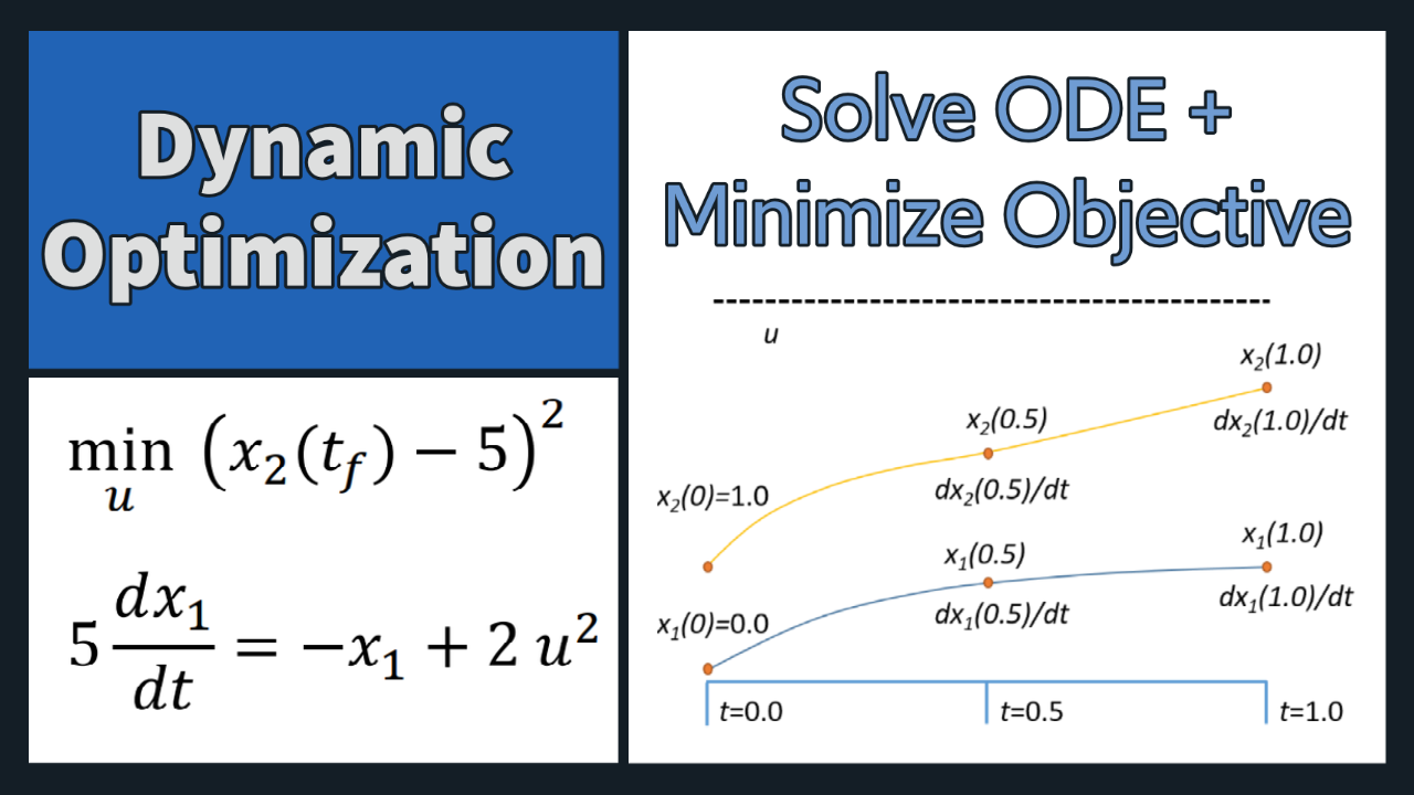
             5*dx11 == -x11 + 2*u**2,
             5*dx12 == -x12 + 2*u**2,
             3*dx21 == -x21 + x11**2,
             3*dx22 == -x22 + x12**2,
             x22-5 == 0])

m.solve(disp=False) print(u[0]) print(x10, x11[0], x12[0]) print(x20, x21[0], x22[0]) print(dx11[0], dx12[0], dx21[0], dx22[0])

from gekko import GEKKO import matplotlib.pyplot as plt import numpy as np

1. Initialize Model

m = GEKKO()

nt = 101 m.time = np.linspace(0,1,nt)

1. Parameters

u = m.MV(value=-6) u.STATUS = 1

1. Variables

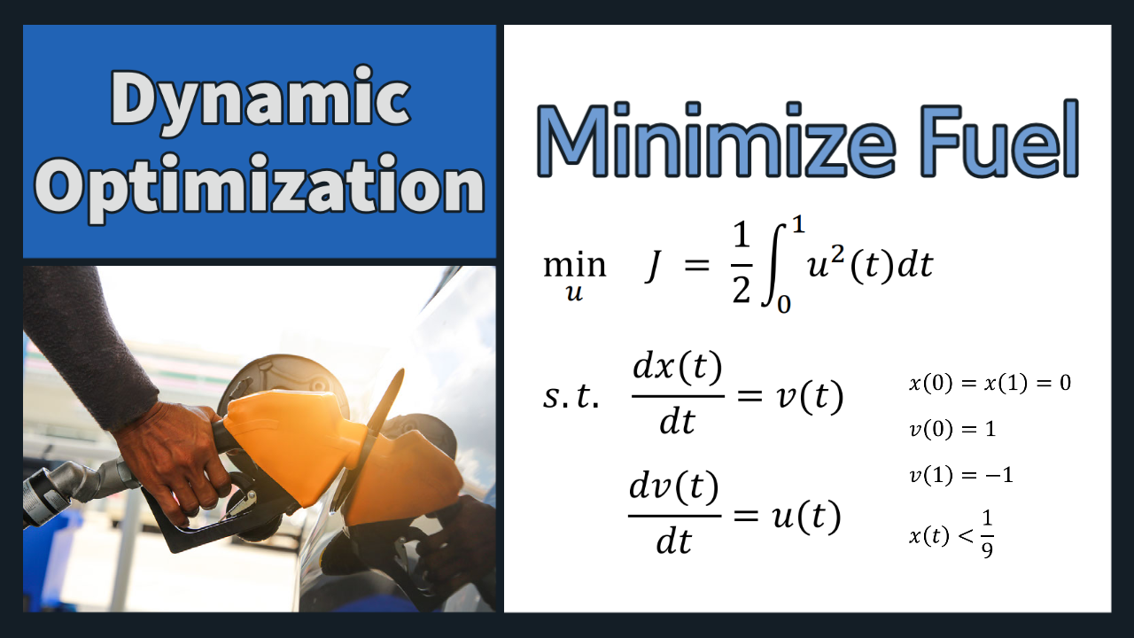
x = m.Var(value=0,ub=1/9) v = m.Var(value=1)

J = m.Intermediate(0.5*m.integral(u**2))

p = np.zeros(nt) p[-1] = 1.0 final = m.Param(value=p)

1. Equations

m.Equation(x.dt() == v) m.Equation(v.dt() == u)

m.Equation(final*x==0) m.Equation(final*(v+1)==0)

1. ,or
2. m.Minimize(final*1e5*x**2)
3. m.Minimize(final*1e5*(v+1)**2)
4. Objective Function

m.Minimize(final*J)

1. Options

m.options.IMODE = 6 m.options.NODES = 2 m.options.SOLVER = 1

m.solve(disp=False)

print('Final Objective Function Value:', J.value[-1])

1. Create a figure

plt.figure(figsize=(10,4)) plt.subplot(2,2,1) plt.plot([0,1],[1/9,1/9],'r:',label=r'$x<\frac{1}{9}$') plt.plot(m.time,x.value,'k-',lw=2,label=r'$x$') plt.ylabel('Position') plt.legend(loc='best') plt.subplot(2,2,2) plt.plot(m.time,v.value,'b--',lw=2,label=r'$v$') plt.ylabel('Velocity') plt.legend(loc='best') plt.subplot(2,2,3) plt.plot(m.time,u.value,'r--',lw=2,label=r'$u$') plt.ylabel('Thrust') plt.legend(loc='best') plt.xlabel('Time') plt.subplot(2,2,4) plt.plot(m.time,J.value,'g-',lw=2,label=r'$\frac{1}{2} \int u^2$') plt.text(0.5,3.0,'Final Value = '+str(np.round(J.value[-1],2))) plt.ylabel('Objective') plt.legend(loc='best') plt.xlabel('Time') plt.show()

import numpy as np from gekko import GEKKO import matplotlib.pyplot as plt

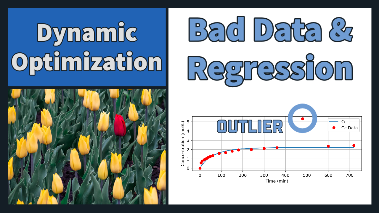
1. data from problem statement

time = np.array([0, 5, 10, 20, 30, 40, 50, 60, 90, 120,

                 150, 180, 240, 300, 360, 480, 600, 720])

Cc_meas = np.array([0,0.57, 0.78, 0.92, 1.04, 1.19, 1.29,

                    1.36, 1.59, 1.68, 1.84, 1.96, 2.01, 2.13,
                    2.21, 5.32, 2.38, 2.44])

m = GEKKO(remote=True)

m.time = time

Kf = m.FV(value =0.0025, lb = 0, ub = 0.01) Kb = m.FV(value =0.0025, lb = 0, ub = 0.01) Kf.STATUS = 1 Kb.STATUS = 1

Ca = m.Var(value = 4.84) Cb = m.Var(value = 9.67) Cd = m.Var(value = 0)

Cc = m.CV(Cc_meas) Cc.FSTATUS = 1

1. Reaction equations

m.Equation(Cc.dt() == Kf*Ca*(Cb**2) - Kb*Cc*Cd) m.Equation(Ca.dt() == -Cc.dt()) m.Equation(Cb.dt() == -2*Cc.dt()) m.Equation(Cd.dt() == Cc.dt())

1. turn GEKKO mode to estimation

m.options.IMODE = 5 m.options.NODES = 4 m.options.EV_TYPE = 1 #2 = Sum of squared error, 1 = Sum of absoluted error

m.solve(disp=False)

1. solve and plot

plt.figure() plt.subplot(2,1,1) plt.plot(m.time, Ca.value, label = 'Ca') plt.plot(m.time, Cb.value, label = 'Cb') plt.ylabel('Concentration (mol/L)') plt.legend(); plt.grid() plt.subplot(2,1,2) plt.plot(m.time, Cc.value, label = 'Cc') plt.plot(m.time, Cc_meas, 'ro', label = 'Cc Data') plt.ylabel('Concentration (mol/L)') plt.xlabel('Time (min)') plt.legend(); plt.grid() plt.ylabel('Concentration (mol/L)') plt.tight_layout() plt.savefig('regression.png',dpi=300)

print("Kf = " + str(Kf.value[0])) print("Kb = " + str(Kb.value[0]))

Problem 2 Solution (Dynamic Optimization)

Problem 2 Solution (Dynamic Optimization Benchmark)

(:title Practice Midterm Exam 3:)

(:title Practice Midterm Exam 3 for Dynamic Optimization:) (:keywords Python, optimal control, outlier, nonlinear control, model predictive control, exam, midterm:) (:description Practice Mid-term exam 3 for dynamic estimation and optimization as a graduate-level course.:)

Midterm Exam 3

Mid-term Exam

Problem 1 Solution (Orthogonal Collocation)

(:toggle hide gekko1 button show="Show Solution Code":) (:div id=gekko1:) (:source lang=python:)

(:sourceend:) (:divend:)

(:html:) (:htmlend:)

Problem 2 Solution (Benchmark)

(:toggle hide gekko2 button show="Show Solution Code":) (:div id=gekko2:) (:source lang=python:)

(:sourceend:) (:divend:)

Problem 3 Solution (Regression with Outlier)

(:toggle hide gekko3 button show="Show Solution Code":) (:div id=gekko3:) (:source lang=python:)

(:sourceend:) (:divend:)