Lotka Volterra Fishing Optimization
Main.LotkaVolterra History
Hide minor edits - Show changes to markup
The differential states `x_0` and `x_1` are the biomass of prey and predator, respectively. The third differential state is the integral of the squared error to drive both the predictor and prey biomass values to 1.0. The decision to send out the fishing fleet at time `t` is the manipulated variable `w(t)`. The time window is from 0 to 12.
The differential states `x_0` and `x_1` are the biomass of prey and predator, respectively. The third differential state is the integral of the squared error to drive both the predator and prey biomass values to 1.0. The decision to send out the fishing fleet at time `t` is the manipulated variable `w(t)`. The time window is from 0 to 12.
(:html:) <iframe width="560" height="315" src="https://www.youtube.com/embed/iwdKOgt9Pnc" frameborder="0" allow="accelerometer; autoplay; clipboard-write; encrypted-media; gyroscope; picture-in-picture" allowfullscreen></iframe> (:htmlend:)
(:keywords preditor, prey, equilibrium, optimization, optimal control, benchmark, nonlinear control, dynamic optimization, engineering optimization, Python, GEKKO, differential, algebraic, modeling language:)
(:keywords predator, prey, equilibrium, optimization, optimal control, benchmark, nonlinear control, dynamic optimization, engineering optimization, Python, GEKKO, differential, algebraic, modeling language:)
The Gekko Optimization Suite is a machine learning and optimization package in Python for mixed-integer and differential algebraic equations. The GEKKO package is available in Python with pip install gekko. There are additional example problems for equation solving, optimization, regression, dynamic simulation, model predictive control, and machine learning.
The Gekko Optimization Suite is a machine learning and optimization package in Python for mixed-integer and differential algebraic equations. The GEKKO package is available in Python with pip install gekko. There are additional example problems for equation solving, optimization, regression, dynamic simulation, model predictive control, and machine learning. Cite Gekko Paper
Avoid Actuator Chatter with Objective Dead-Band
Avoid Actuator Chatter
Reference
Reference
The differential states `x_0` and `x_1` are the biomass of prey and predator, respectively. The third differential state is the integral of the squared error to drive both the predictor and prey biomass values to 1.0. The decision to send out the fishing fleet at time `t` is the manipulated variable `w(t)`. The time window is from 0 to 12 and the parameters have values `c_1=0.4` and `c_2=0.2`.
The differential states `x_0` and `x_1` are the biomass of prey and predator, respectively. The third differential state is the integral of the squared error to drive both the predictor and prey biomass values to 1.0. The decision to send out the fishing fleet at time `t` is the manipulated variable `w(t)`. The time window is from 0 to 12.
Reference
- Sager, S., Bock, H.G., Diehl, M., Reinelt, G., Schloder, J.P. (2006). Numerical Methods for Optimal Control with Binary Control Functions Applied to a Lotka-Volterra Type Fishing Problem. In: Seeger, A. (eds) Recent Advances in Optimization. Lecture Notes in Economics and Mathematical Systems, vol 563. Springer, Berlin, Heidelberg. https://doi.org/10.1007/3-540-28258-0_17
(:toggle hide solution button show="Lotka Volterra Source":)
(:toggle hide solution button show="🐍 Lotka Volterra Python Source":)
(:toggle hide solution2 button show="Dead-band MPC Source":)
(:toggle hide solution2 button show="🐍 Dead-band MPC Python Source":)
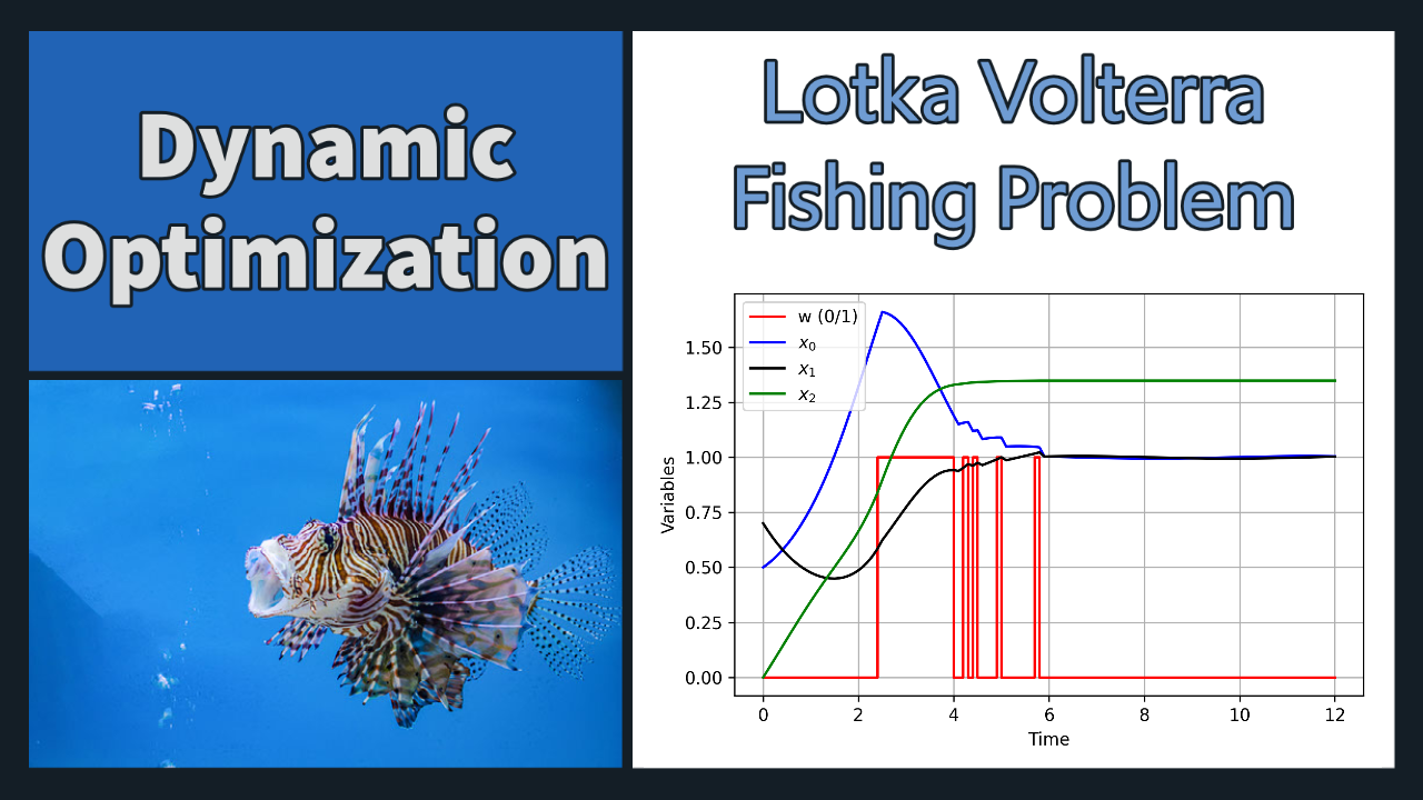
The Lotka Volterra fishing problem seeks an optimal fishing strategy over a fixed time horizon to bring both predator and prey fish to a desired steady state. The manipulted variable is the fishing by man. The manipulated variable is either continuous or a discrete value with no fishing (0) or full fishing (1).
The Lotka Volterra fishing problem seeks an optimal fishing strategy over a fixed time horizon to bring both predator and prey fish to a desired steady state. The manipulated variable is the fishing by man. The manipulated variable is either continuous or a discrete value with no fishing (0) or full fishing (1).
Avoid Actuator Chatter with Objective Dead-Band
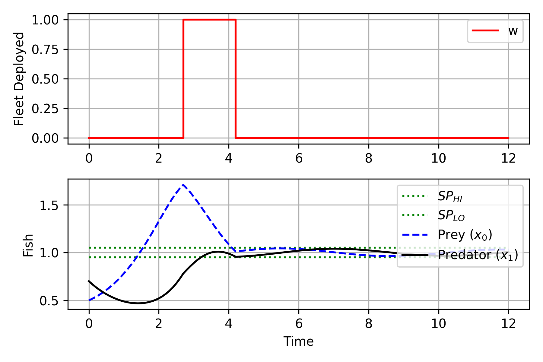
The solution with a squared objective has chatter in the fishing decision variable w as the fishing fleet is deployed and returns repeatedly to achieve a perfect balance between predator and prey. This repeated action can wear out an actuator such as a valve that is quickly switched open or closed or a motor that switched on or off. The fishing fleet deployment schedule would also have additional costs for the fishermen and logistics to implement the schedule. A potential improvement is to set up a dead-band around the objective or to include actuator move-suppression. A dead-band of +/-0.05 is set around the objective of 1.0 so that 0.95 to 1.05 are acceptable for the predator and prey levels.
(:toggle hide solution2 button show="Dead-band MPC Source":) (:div id=solution2:) (:source lang=python:) import numpy as np import matplotlib.pyplot as plt from gekko import GEKKO
m = GEKKO(remote=True)
- Add 0.01 as first step
- 0,0.01,0.1,0.2,0.3,...11.9,12.0)
m.time = np.insert(np.linspace(0,12,121),1,0.01)
- change solver options
m.solver_options = ['minlp_gap_tol 0.001', 'minlp_maximum_iterations 10000', 'minlp_max_iter_with_int_sol 30', 'minlp_branch_method 3', 'minlp_integer_tol 0.001', 'minlp_integer_leaves 0', 'minlp_maximum_iterations 200']
c0 = 0.4; c1 = 0.2
last = m.Param(np.zeros(122)) last.value[-1] = 1
x0 = m.CV(value=0.5,lb=0) x0.STATUS = 1; x0.SPHI=1.05; x0.SPLO=0.95 x1 = m.CV(value=0.7,lb=0) x1.STATUS = 1; x1.SPHI=1.05; x1.SPLO=0.95
w = m.MV(value=0,lb=0,ub=1,integer=True) w.STATUS = 1
m.Equations([x0.dt() == x0 - x0*x1 - c0*x0*w, x1.dt() == - x1 + x0*x1 - c1*x1*w])
m.options.IMODE = 6 m.options.NODES = 2 m.options.SOLVER = 1 m.options.MV_TYPE = 0 m.solve()
plt.figure(figsize=(6,4)) plt.subplot(2,1,1) plt.step(m.time,w.value,'r-',label='w') plt.legend(loc=1); plt.grid(); plt.ylabel('Fleet Deployed') plt.subplot(2,1,2) plt.plot([0,12],[1.05,1.05],'g:',label=r'$SP_{HI}$') plt.plot([0,12],[0.95,0.95],'g:',label=r'$SP_{LO}$') plt.plot(m.time,x0.value,'b-',label=r'Prey $(x_0)$') plt.plot(m.time,x1.value,'k-',label=r'Predator $(x_1)$') plt.xlabel('Time'); plt.ylabel('Fish') plt.legend(loc=1); plt.grid(); plt.tight_layout() plt.savefig('lotka2.png',dpi=300); plt.show() (:sourceend:) (:divend:)
$$\quad \quad \frac{dx_2}{dt} = \left(x_0-1\right)^2 + \left(x_1-1\right)^2$$
$$\quad \quad x_2 = \int_0^{t_f} \left(x_0-1\right)^2 + \left(x_1-1\right)^2 dt$$
The differential states `x_0` and `x_1` are the biomass of prey and predator, respectively. The third differential state is the integral of the objective to drive both the predictor and prey biomass values to 1.0. The decision to send out the fishing fleet at time `t` is the decision variable `w(t)`. The time window is from 0 to 12 and the parameters have values `c_1=0.4` and `c_2=0.2`.
The differential states `x_0` and `x_1` are the biomass of prey and predator, respectively. The third differential state is the integral of the squared error to drive both the predictor and prey biomass values to 1.0. The decision to send out the fishing fleet at time `t` is the manipulated variable `w(t)`. The time window is from 0 to 12 and the parameters have values `c_1=0.4` and `c_2=0.2`.
A Mixed Integer Optimal Control Problem (MIOCP) is the Lotka Volterra fishing problem. It finds an fishing strategy over 12 years to equilibrate the predator-prey fish to a sustainable steady-state value. The Lotka Volterra equations for a predator-prey system have an additional term to introduce fishing by man with constants `c_0=0.4` and `c_1=0.2`.
The Lotka Volterra fishing problem is a Mixed Integer Optimal Control Problem (MIOCP). It finds a fishing strategy over 12 years to equilibrate the predator-prey fish to a sustainable steady-state value. The Lotka Volterra equations for a predator-prey system have an additional term to introduce fishing by man with constants `c_0=0.4` and `c_1=0.2`.
The Gekko Optimization Suite is a machine learning and optimization package in Python for mixed-integer and differential algebraic equations. The GEKKO package is available in Python with pip install gekko. There are additional example problems? for equation solving, optimization, regression, dynamic simulation, model predictive control, and machine learning.
The Gekko Optimization Suite is a machine learning and optimization package in Python for mixed-integer and differential algebraic equations. The GEKKO package is available in Python with pip install gekko. There are additional example problems for equation solving, optimization, regression, dynamic simulation, model predictive control, and machine learning.
The differential states `x_0` and `x_1` are the biomass of prey and predator, respectively. The third differential state is the integral of the objective to drive both the predictor and prey biomass values to 1.0. The decision to send out the fishing fleet at time `t` is the decision variable `w(t)`. The time window is from 0 to 12 and the parameters have values `c_1=0.4` and `c_2=0.2`.
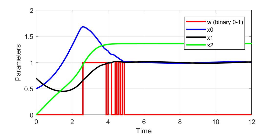
The mathematical equations are Ordinary Differential Equations (ODEs). The optimal binary manipulated variable chatters on and off, making the Lotka Volterra fishing problem an interesting benchmark of mixed-integer optimal control solvers. The mixed-integer optimal control problem is given by
$$ \begin{array}{llclr} \min_{x,w} & x_2(t_f) \\ \mbox{s.t.} & \dot{x}_0 & = & x_0 - x_0 x_1 - \; c_0 x_0 \; w \\ & \dot{x}_1 & = & - x_1 + x_0 x_1 - \; c_1 x_1 \; w \\ & \dot{x}_2 & = & (x_0 - 1)^2 + (x_1 - 1)^2 \\ & x(0) &=& (0.5, 0.7, 0)^T \\ & w(t) &\in& \{0, 1\} \end{array} $$
The differential states `x_0` and `x_1` are the biomass of prey and predator, respectively. The third differential state is the integral of the objective to drive both the predictor and prey biomass values to 1.0. The decision to send out the fishing fleet at time `t` is the decision variable `w(t)`. The time window is from 0 to 12 and the parameters have values `c_1=0.4` and `c_2=0.2`.
The mathematical equations are Ordinary Differential Equations (ODEs). The optimal binary manipulated variable chatters on and off, making the Lotka Volterra fishing problem an interesting benchmark of mixed-integer optimal control solvers.
$$ \begin{array}{llclr} \min_{x, w} & x_2(t_f) \\ \mbox{s.t.} & \dot{x}_0 & = & x_0 - x_0 x_1 - \; c_0 x_0 \; w \\ & \dot{x}_1 & = & - x_1 + x_0 x_1 - \; c_1 x_1 \; w \\ & \dot{x}_2 & = & (x_0 - 1)^2 + (x_1 - 1)^2 \\ & x(0) &=& (0.5, 0.7, 0)^T \\ & w(t) &\in& \{0, 1\} \end{array} $$
$$ \begin{array}{llclr} \min_{x,w} & x_2(t_f) \\ \mbox{s.t.} & \dot{x}_0 & = & x_0 - x_0 x_1 - \; c_0 x_0 \; w \\ & \dot{x}_1 & = & - x_1 + x_0 x_1 - \; c_1 x_1 \; w \\ & \dot{x}_2 & = & (x_0 - 1)^2 + (x_1 - 1)^2 \\ & x(0) &=& (0.5, 0.7, 0)^T \\ & w(t) &\in& \{0, 1\} \end{array} $$
(:title Lotka Volterra Fishing Optimization:) (:keywords preditor, prey, equilibrium, optimization, optimal control, benchmark, nonlinear control, dynamic optimization, engineering optimization, Python, GEKKO, differential, algebraic, modeling language:) (:description The Lotka Volterra fishing problem solved with Python Gekko.:)
lotka_volterra.png
A Mixed Integer Optimal Control Problem (MIOCP) is the Lotka Volterra fishing problem. It finds an fishing strategy over 12 years to equilibrate the predator-prey fish to a sustainable steady-state value. The Lotka Volterra equations for a predator-prey system have an additional term to introduce fishing by man with constants `c_0=0.4` and `c_1=0.2`.
$$\min_{x,w} x_2 \left( t_f \right)$$
$$\mathrm{s.t.} \quad \frac{dx_0}{dt} = x_0 - x_0 x_1 - c_0 x_0 w$$ $$\quad \quad \frac{dx_1}{dt} = -x_1 + x_0 x_1 - c_1 x_1 w$$ $$\quad \quad \frac{dx_2}{dt} = \left(x_0-1\right)^2 + \left(x_1-1\right)^2$$ $$\quad \quad x(0) = (0.5,0.7,0)^T$$ $$\quad \quad w(t) \in {{0,1}}$$
The Lotka Volterra fishing problem seeks an optimal fishing strategy over a fixed time horizon to bring both predator and prey fish to a desired steady state. The manipulted variable is the fishing by man. The manipulated variable is either continuous or a discrete value with no fishing (0) or full fishing (1).
The mathematical equations are Ordinary Differential Equations (ODEs). The optimal binary manipulated variable chatters on and off, making the Lotka Volterra fishing problem an interesting benchmark of mixed-integer optimal control solvers. The mixed-integer optimal control problem is given by
$$ \begin{array}{llclr} \min_{x, w} & x_2(t_f) \\ \mbox{s.t.} & \dot{x}_0 & = & x_0 - x_0 x_1 - \; c_0 x_0 \; w \\ & \dot{x}_1 & = & - x_1 + x_0 x_1 - \; c_1 x_1 \; w \\ & \dot{x}_2 & = & (x_0 - 1)^2 + (x_1 - 1)^2 \\ & x(0) &=& (0.5, 0.7, 0)^T \\ & w(t) &\in& \{0, 1\} \end{array} $$
The differential states `x_0` and `x_1` are the biomass of prey and predator, respectively. The third differential state is the integral of the objective to drive both the predictor and prey biomass values to 1.0. The decision to send out the fishing fleet at time `t` is the decision variable `w(t)`. The time window is from 0 to 12 and the parameters have values `c_1=0.4` and `c_2=0.2`.
(:toggle hide solution button show="Lotka Volterra Source":) (:div id=solution:) (:source lang=python:) import numpy as np import matplotlib.pyplot as plt from gekko import GEKKO
m = GEKKO(remote=False)
- Add 0.01 as first step
- 0,0.01,0.1,0.2,0.3,...11.9,12.0)
m.time = np.insert(np.linspace(0,12,121),1,0.01)
- change solver options
m.solver_options = ['minlp_gap_tol 0.001', 'minlp_maximum_iterations 10000', 'minlp_max_iter_with_int_sol 100', 'minlp_branch_method 1', 'minlp_integer_tol 0.001', 'minlp_integer_leaves 0', 'minlp_maximum_iterations 200']
c0 = 0.4; c1 = 0.2
last = m.Param(np.zeros(122)) last.value[-1] = 1
x0 = m.Var(value=0.5,lb=0) x1 = m.Var(value=0.7,lb=0) x2 = m.Var(value=0.0,lb=0) w = m.MV(value=0,lb=0,ub=1,integer=True) w.STATUS = 1
m.Minimize(last*x2)
m.Equations([x0.dt() == x0 - x0*x1 - c0*x0*w, x1.dt() == - x1 + x0*x1 - c1*x1*w, x2 == m.integral((x0-1)**2 + (x1-1)**2)])
m.options.IMODE = 6 m.options.NODES = 3 m.options.SOLVER = 1 m.options.MV_TYPE = 0 m.solve()
plt.figure(figsize=(6,4)) plt.step(m.time,w.value,'r-',label='w (0/1)') plt.plot(m.time,x0.value,'b-',label=r'$x_0$') plt.plot(m.time,x1.value,'k-',label=r'$x_1$') plt.plot(m.time,x2.value,'g-',label=r'$x_2$') plt.xlabel('Time'); plt.ylabel('Variables') plt.legend(loc='best'); plt.grid(); plt.tight_layout() plt.savefig('lotka.png',dpi=300); plt.show() (:sourceend:) (:divend:)

An MINLP solution is calculated with APOPT with an objective function value of `x_2(t_f) = 1.3495`.

The Gekko Optimization Suite is a machine learning and optimization package in Python for mixed-integer and differential algebraic equations. The GEKKO package is available in Python with pip install gekko. There are additional example problems? for equation solving, optimization, regression, dynamic simulation, model predictive control, and machine learning.