Deep Learning
Main.DeepLearning History
Hide minor edits - Show changes to markup
plt.show() (:sourceend:) (:divend:)
(:toggle hide sklearn button show="Show Python Scikit-Learn Example Code":) (:div id=sklearn:)
(:source lang=python:) from sklearn.neural_network import MLPRegressor import numpy as np import matplotlib.pyplot as plt
- generate training data
x = np.linspace(0.0,2*np.pi) xr = x.reshape(-1,1) y = np.sin(x)
- train
nn = MLPRegressor(hidden_layer_sizes=(3),
activation='tanh', solver='lbfgs',max_iter=2000)
model = nn.fit(xr,y)
- validate
xp = np.linspace(-2*np.pi,4*np.pi,100) xpr = xp.reshape(-1,1) yp = nn.predict(xpr) ypr = yp.reshape(-1,1) r2 = nn.score(xpr,ypr) print('R^2: ' + str(r2))
plt.figure() plt.plot(x,y,'bo') plt.plot(xpr,ypr,'r-')
b = brain.Brain(1)
b = brain.Brain()
(:toggle hide gekko_brain button show="Show Python Gekko Example Code":) (:div id=gekko_brain:)
(:source lang=python:) from gekko import brain import numpy as np import matplotlib.pyplot as plt
- generate training data
x = np.linspace(0.0,2*np.pi) y = np.sin(x)
b = brain.Brain(1) b.input_layer(1) b.layer(linear=2) b.layer(tanh=2) b.layer(linear=2) b.output_layer(1)
- train
b.learn(x,y)
- validate
xp = np.linspace(-2*np.pi,4*np.pi,100) yp = b.think(xp)
plt.figure() plt.plot(x,y,'bo') plt.plot(xp,yp[0],'r-') plt.show() (:sourceend:) (:divend:)
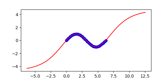
Repeat the above exercise that was shown with Keras with Python Gekko. Change the activation function to a cosine to better extrapolate outside of the training region. The training data are 20 equally spaced points for x between 0 and `2\pi` with outputs generated from the sine function `y = \sin(x)`.
Repeat the above exercise that was shown with Keras with Python Gekko but change the activation function to a cosine to better extrapolate outside of the training region. The training data are 20 equally spaced points for x between 0 and `2\pi` with outputs generated from the sine function `y = \sin(x)`.
<video controls autoplay loop>
  <source src="/do/uploads/Main/keras_tutorial.mp4" type="video/mp4">
  Your browser does not support the video tag.
</video>
<iframe width="560" height="315" src="https://www.youtube.com/embed/zOCVTPb5DiM" frameborder="0" allow="accelerometer; autoplay; encrypted-media; gyroscope; picture-in-picture" allowfullscreen></iframe>
(:html:) <video controls autoplay loop>
  <source src="/do/uploads/Main/keras_tutorial.mp4" type="video/mp4">
  Your browser does not support the video tag.
</video> (:htmlend:)
Repeat the above exercise that was shown with Keras with Python Gekko.
Change the activation function to a cosine to better extrapolate outside of the training region. The training data are 20 equally spaced points for x between 0 and `2\pi` with outputs generated from the sine function `y = \sin(x)`.
Repeat the above exercise that was shown with Keras with Python Gekko. Change the activation function to a cosine to better extrapolate outside of the training region. The training data are 20 equally spaced points for x between 0 and `2\pi` with outputs generated from the sine function `y = \sin(x)`.
- Generate Data ###############################################
- Scale data ##################################################
- Train model #################################################
- Test model ##################################################
- Predictions Outside Training Region #########################
<video controls autoplay>
<video controls autoplay loop>
<source src="/uploads/Main/keras_tutorial.mp4" type="video/mp4">
<source src="/do/uploads/Main/keras_tutorial.mp4" type="video/mp4">
(:html:) <video controls autoplay>
  <source src="/uploads/Main/keras_tutorial.mp4" type="video/mp4">
  Your browser does not support the video tag.
</video> (:htmlend:)
Repeat the above exercise that was shown with Keras with Python Gekko. Change the activation function to a cosine to better extrapolate outside of the training region. The training data are 20 equally spaced points for x between 0 and `2\pi` with outputs generated from the sine function `y = \sin(x)`.
Repeat the above exercise that was shown with Keras with Python Gekko.
Change the activation function to a cosine to better extrapolate outside of the training region. The training data are 20 equally spaced points for x between 0 and `2\pi` with outputs generated from the sine function `y = \sin(x)`.
Two applications of deep learning are regression (predict outcome) and classification (distinguish among discrete options). In each case, there is training data that is used to adjust weights (unknown parameters) that minimize a loss function (objective function). A trained model is useful to predict outcomes based on new input conditions that aren't in the original data set. Some of the typical steps for building and deploying a deep learning application are data consolidation, data cleansing, model building, training, validation, and deployment. Example Python code is provided for each of the steps.
Two applications of deep learning are regression (predict outcome) and classification (distinguish among discrete options). In each case, there is training data that is used to adjust weights (unknown parameters) that minimize a loss function (objective function).
A trained model predicts outcomes based on new input conditions that aren't in the original data set. Some of the typical steps for building and deploying a deep learning application are data consolidation, data cleansing, model building, training, validation, and deployment. Example Python code is provided for each of the steps.
(:html:) <iframe width="560" height="315" src="https://www.youtube.com/embed/kOmhU2XxLCY" frameborder="0" allow="accelerometer; autoplay; encrypted-media; gyroscope; picture-in-picture" allowfullscreen></iframe> (:htmlend:)
(:toggle hide solution button show="Show All Keras Example Code":)
(:toggle hide keras button show="Show All Keras Example Code":)
(:toggle hide solution button show="Show Python Gekko Source":)
(:toggle hide gekko button show="Show Python Gekko Source":)
plt.legend(loc='best')
(:sourceend:)
plt.show() (:sourceend:)
(:toggle hide solution button show="Show All Keras Example Code":) (:div id=keras:) (:source lang=python:) import numpy as np import pandas as pd from sklearn.preprocessing import MinMaxScaler from keras.models import Sequential from keras.layers import * import matplotlib.pyplot as plt
- Generate Data ###############################################
- generate training data
x = np.linspace(0.0,2*np.pi,20) y = np.sin(x)
- save training data to file
data = np.vstack((x,y)).T np.savetxt('train_data.csv',data,header='x,y',comments='',delimiter=',')
- generate test data
x = np.linspace(0.0,2*np.pi,100) y = np.sin(x)
- save test data to file
data = np.vstack((x,y)).T np.savetxt('test_data.csv',data,header='x,y',comments='',delimiter=',')
- Scale data ##################################################
- load training and test data with pandas
train_df = pd.read_csv('train_data.csv') test_df = pd.read_csv('test_data.csv')
- scale values to 0 to 1 for the ANN to work well
s = MinMaxScaler(feature_range=(0,1))
- scale training and test data
sc_train = s.fit_transform(train_df) sc_test = s.transform(test_df)
- print scaling adjustments
print('Scalar multipliers') print(s.scale_) print('Scalar minimum') print(s.min_)
- convert scaled values back to dataframe
sc_train_df = pd.DataFrame(sc_train, columns=train_df.columns.values) sc_test_df = pd.DataFrame(sc_test, columns=test_df.columns.values)
- save scaled values to CSV files
sc_train_df.to_csv('train_scaled.csv', index=False) sc_test_df.to_csv('test_scaled.csv', index=False)
- Train model #################################################
- create neural network model
model = Sequential() model.add(Dense(1, input_dim=1, activation='linear')) model.add(Dense(2, activation='linear')) model.add(Dense(2, activation='tanh')) model.add(Dense(2, activation='linear')) model.add(Dense(1, activation='linear')) model.compile(loss="mean_squared_error", optimizer="adam")
- load training data
train_df = pd.read_csv("train_scaled.csv") X1 = train_df.drop('y', axis=1).values Y1 = train_df'y'?.values
- train the model
model.fit(X1,Y1,epochs=5000,verbose=0,shuffle=True)
- Save the model to hard drive
- model.save('model.h5')
- Test model ##################################################
- Load the model from hard drive
- model.load('model.h5')
- load test data
test_df = pd.read_csv("test_scaled.csv") X2 = test_df.drop('y', axis=1).values Y2 = test_df'y'?.values
- test the model
mse = model.evaluate(X2,Y2, verbose=1)
print('Mean Squared Error: ', mse)
- Predictions Outside Training Region #########################
- generate prediction data
x = np.linspace(-2*np.pi,4*np.pi,100) y = np.sin(x)
- scale input
X3 = x*s.scale_[0]+s.min_[0]
- predict
Y3P = model.predict(X3)
- unscale output
yp = (Y3P-s.min_[1])/s.scale_[1]
plt.figure() plt.plot((X1-s.min_[0])/s.scale_[0], (Y1-s.min_[1])/s.scale_[1], 'bo',label='train') plt.plot(x,y,'r-',label='actual') plt.plot(x,yp,'k--',label='predict') plt.legend(loc='best') plt.savefig('results.png') plt.show() (:sourceend:) (:divend:)
Exercise
Repeat the above exercise that was shown with Keras with Python Gekko. Change the activation function to a cosine to better extrapolate outside of the training region. The training data are 20 equally spaced points for x between 0 and `2\pi` with outputs generated from the sine function `y = \sin(x)`.
(:toggle hide solution button show="Show Python Gekko Source":) (:div id=gekko:) (:source lang=python:) from gekko import GEKKO import numpy as np import matplotlib.pyplot as plt
- generate training data
x = np.linspace(0.0,2*np.pi,20) y = np.sin(x)
- option for fitting function
select = True # True / False if select:
    # Size with cosine function
    nin = 1  # inputs
    n1 = 1   # hidden layer 1 (linear)
    n2 = 1   # hidden layer 2 (nonlinear)
    n3 = 1   # hidden layer 3 (linear)
    nout = 1 # outputs
else:
    # Size with hyperbolic tangent function
    nin = 1  # inputs
    n1 = 2   # hidden layer 1 (linear)
    n2 = 2   # hidden layer 2 (nonlinear)
    n3 = 2   # hidden layer 3 (linear)
    nout = 1 # outputs
- Initialize gekko
train = GEKKO() test = GEKKO()
model = [train,test]
for m in model:
    # input(s)
    m.inpt = m.Param()

    # layer 1
    m.w1 = m.Array(m.FV, (nin,n1))
    m.l1 = [m.Intermediate(m.w1[0,i]*m.inpt) for i in range(n1)]

    # layer 2
    m.w2a = m.Array(m.FV, (n1,n2))
    m.w2b = m.Array(m.FV, (n1,n2))
    if select:
        m.l2 = [m.Intermediate(sum([m.cos(m.w2a[j,i]+m.w2b[j,i]*m.l1[j])                                 for j in range(n1)])) for i in range(n2)]
    else:
        m.l2 = [m.Intermediate(sum([m.tanh(m.w2a[j,i]+m.w2b[j,i]*m.l1[j])                                 for j in range(n1)])) for i in range(n2)]

    # layer 3
    m.w3 = m.Array(m.FV, (n2,n3))
    m.l3 = [m.Intermediate(sum([m.w3[j,i]*m.l2[j]             for j in range(n2)])) for i in range(n3)]

    # output(s)
    m.outpt = m.CV()
    m.Equation(m.outpt==sum([m.l3[i] for i in range(n3)]))

    # flatten matrices
    m.w1 = m.w1.flatten()
    m.w2a = m.w2a.flatten()
    m.w2b = m.w2b.flatten()
    m.w3 = m.w3.flatten()
- Fit parameter weights
m = train m.inpt.value=x m.outpt.value=y m.outpt.FSTATUS = 1 for i in range(len(m.w1)):
    m.w1[i].FSTATUS=1
    m.w1[i].STATUS=1
    m.w1[i].MEAS=1.0
for i in range(len(m.w2a)):
    m.w2a[i].STATUS=1
    m.w2b[i].STATUS=1
    m.w2a[i].FSTATUS=1
    m.w2b[i].FSTATUS=1
    m.w2a[i].MEAS=1.0
    m.w2b[i].MEAS=0.5
for i in range(len(m.w3)):
    m.w3[i].FSTATUS=1
    m.w3[i].STATUS=1
    m.w3[i].MEAS=1.0
m.options.IMODE = 2 m.options.SOLVER = 3 m.options.EV_TYPE = 2 m.solve(disp=False)
- Test sample points
m = test for i in range(len(m.w1)):
    m.w1[i].MEAS=train.w1[i].NEWVAL
    m.w1[i].FSTATUS = 1
    print('w1[str(i)]: '+str(m.w1[i].MEAS))
for i in range(len(m.w2a)):
    m.w2a[i].MEAS=train.w2a[i].NEWVAL
    m.w2b[i].MEAS=train.w2b[i].NEWVAL
    m.w2a[i].FSTATUS = 1
    m.w2b[i].FSTATUS = 1
    print('w2a[str(i)]: '+str(m.w2a[i].MEAS))
    print('w2b[str(i)]: '+str(m.w2b[i].MEAS))
for i in range(len(m.w3)):
    m.w3[i].MEAS=train.w3[i].NEWVAL
    m.w3[i].FSTATUS = 1
    print('w3[str(i)]: '+str(m.w3[i].MEAS))
m.inpt.value=np.linspace(-2*np.pi,4*np.pi,100) m.options.IMODE = 2 m.options.SOLVER = 3 m.solve(disp=False)
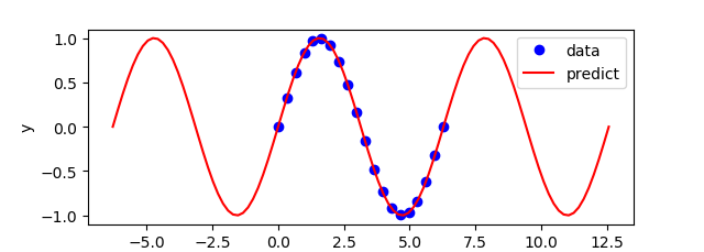
plt.figure() plt.plot(x,y,'bo',label='data') plt.plot(test.inpt.value,test.outpt.value,'r-',label='predict') plt.legend(loc='best') plt.ylabel('y') plt.xlabel('x') plt.show() (:sourceend:) (:divend:)
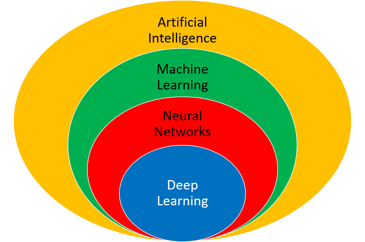
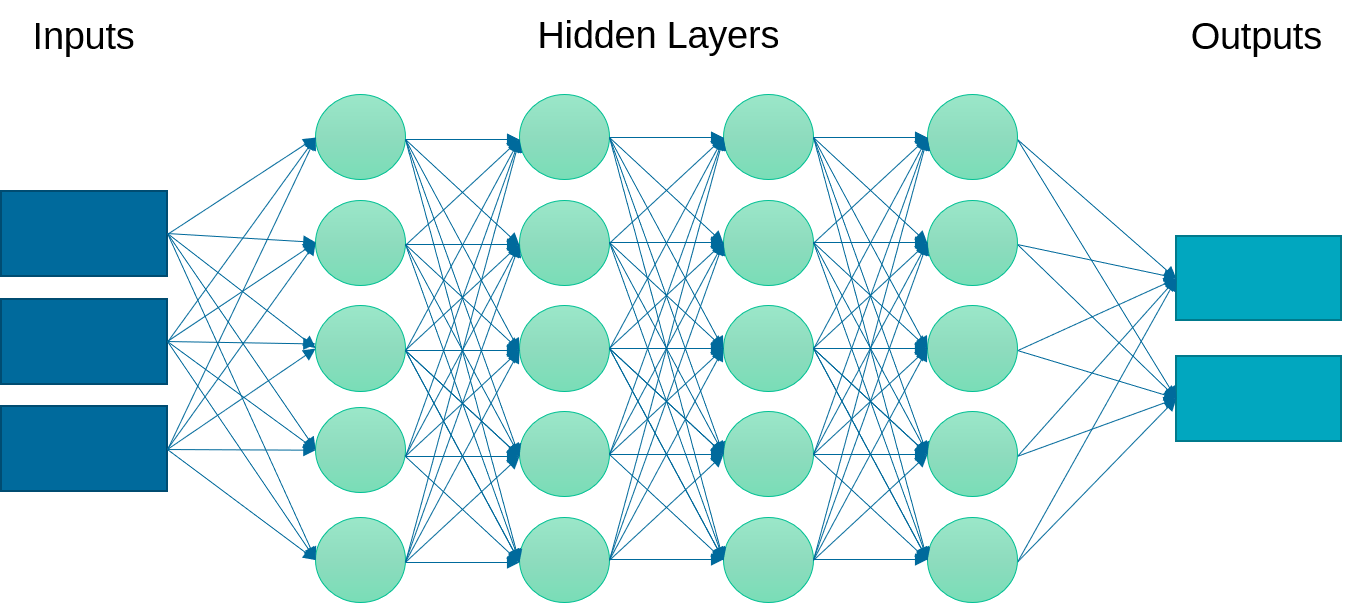
The deep learning algorithm uses a multi-layered neural network. This neural network may have linear or nonlinear layers. The layer form is determined by the type of activation function (e.g. linear, rectified linear unit (ReLU), hyperbolic tangent) that transforms each intermediate input to the next layer.
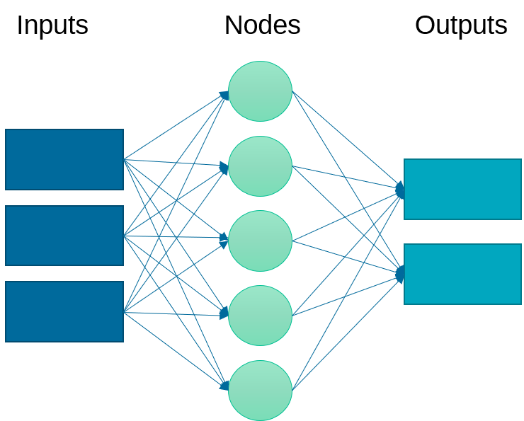
An artificial neural network relates inputs to outputs with layers of nodes. There nodes are also called neurons because they emulate the learning process that occurs in the brain where the connection strength is adjusted to change the learned outcome.
Instead of just one layer, deep learning uses a multi-layered neural network. This neural network may have linear or nonlinear layers. The layer form is determined by the type of activation function (e.g. linear, rectified linear unit (ReLU), hyperbolic tangent) that transforms each intermediate input to the next layer.
Two applications of deep learning are regression (predict outcome) and classification (distinguish among discrete options). In each case, there is training data that is used to adjust weights (unknown parameters) that minimize a loss function (objective function). A trained model is useful to predict outcomes based on new input conditions that aren't in the original data set. Some of the typical steps for building and deploying a deep learning application are (1) data cleansing, (2), model build, (3) training, (4) validation, and (5) deployment.
Two applications of deep learning are regression (predict outcome) and classification (distinguish among discrete options). In each case, there is training data that is used to adjust weights (unknown parameters) that minimize a loss function (objective function). A trained model is useful to predict outcomes based on new input conditions that aren't in the original data set. Some of the typical steps for building and deploying a deep learning application are data consolidation, data cleansing, model building, training, validation, and deployment. Example Python code is provided for each of the steps.
Data Export with Numpy / Import with Pandas
1. Data Export with Numpy / Import with Pandas
Data Scaling with scikit-learn
2. Data Scaling with scikit-learn
Model Build and Train with Keras
3. Model Build and Train with Keras
Model Validation with Keras
4. Model Validation with Keras
Model Predictions with Keras
5. Model Predictions with Keras
Data Export with Numpy / Import with Pandas
Data Scaling with scikit-learn
(:source lang=python:)
- Scale data ##################################################
- load training and test data with pandas
train_df = pd.read_csv('train_data.csv') test_df = pd.read_csv('test_data.csv')
- scale values to 0 to 1 for the ANN to work well
s = MinMaxScaler(feature_range=(0,1))
- scale training and test data
sc_train = s.fit_transform(train_df) sc_test = s.transform(test_df)
- print scaling adjustments
print('Scalar multipliers') print(s.scale_) print('Scalar minimum') print(s.min_)
- convert scaled values back to dataframe
sc_train_df = pd.DataFrame(sc_train, columns=train_df.columns.values) sc_test_df = pd.DataFrame(sc_test, columns=test_df.columns.values)
- save scaled values to CSV files
sc_train_df.to_csv('train_scaled.csv', index=False) sc_test_df.to_csv('test_scaled.csv', index=False) (:sourceend:)
Model Build and Train with Keras
(:source lang=python:)
- Train model #################################################
- create neural network model
model = Sequential() model.add(Dense(1, input_dim=1, activation='linear')) model.add(Dense(2, activation='linear')) model.add(Dense(2, activation='tanh')) model.add(Dense(2, activation='linear')) model.add(Dense(1, activation='linear')) model.compile(loss="mean_squared_error", optimizer="adam")
- load training data
train_df = pd.read_csv("train_scaled.csv") X1 = train_df.drop('y', axis=1).values Y1 = train_df'y'?.values
- train the model
model.fit(X1,Y1,epochs=5000,verbose=0,shuffle=True)
- Save the model to hard drive
- model.save('model.h5')
(:sourceend:)
Model Validation with Keras
(:source lang=python:)
- Test model ##################################################
- Load the model from hard drive
- model.load('model.h5')
- load test data
test_df = pd.read_csv("test_scaled.csv") X2 = test_df.drop('y', axis=1).values Y2 = test_df'y'?.values
- test the model
mse = model.evaluate(X2,Y2, verbose=1)
print('Mean Squared Error: ', mse) (:sourceend:)
Model Predictions with Keras
(:source lang=python:)
- Predictions Outside Training Region #########################
- generate prediction data
x = np.linspace(-2*np.pi,4*np.pi,100) y = np.sin(x)
- scale input
X3 = x*s.scale_[0]+s.min_[0]
- predict
Y3P = model.predict(X3)
- unscale output
yp = (Y3P-s.min_[1])/s.scale_[1]
plt.figure() plt.plot((X1-s.min_[0])/s.scale_[0], (Y1-s.min_[1])/s.scale_[1], 'bo',label='train') plt.plot(x,y,'r-',label='actual') plt.plot(x,yp,'k--',label='predict') plt.savefig('results.png') (:sourceend:)
(:keywords big data, artificial intelligence, machine learning, tutorial, tensorflow, keras:) (:description Deep learning is an application of machine learning with a multi-layered neural network. It is one of many machine learning methods for synthesizing data into a predictive form.:)
(:keywords big data, artificial intelligence, machine learning, tutorial, tensorflow, keras, gekko:) (:description Deep learning is a type of machine learning with a multi-layered neural network. It is one of many machine learning methods for synthesizing data into a predictive form.:)
Deep learning is a type of machine learning with a multi-layered neural network. It is one of many machine learning methods for synthesizing data into a predictive form.
Exercise
Two applications of deep learning are regression (predict outcome) and classification (distinguish among discrete options). In each case, there is training data that is used to adjust weights (unknown parameters) that minimize a loss function (objective function). A trained model is useful to predict outcomes based on new input conditions that aren't in the original data set. Some of the typical steps for building and deploying a deep learning application are (1) data cleansing, (2), model build, (3) training, (4) validation, and (5) deployment.
Data Preparation
- Consolidation - consolidation is the process of combining disparate data (Excel spreadsheet, PDF report, database, cloud storage) into a single repository.
- Data Cleansing - bad data should be removed and may include outliers, missing entries, failed sensors, or other types of missing or corrupted information.
- Inputs and Outputs - data is separated into inputs (explanatory variables) and outputs (supervisory signal). The inputs will be fed into a series of functions to produce an output prediction. The squared difference between the predicted output and the measured output is a typical loss (objective) function for fitting.
- Scaling - scaling all data (inputs and outputs) to a range of 0-1 can improve the training process.
- Training and Validation - data is divided into training (e.g. 80%) and validation (e.g. 20%) sets so that the model fit can be evaluated independently of the training. Cross-validation is an approach to divide the training data into multiple sets that are fit separately. The parameter consistency is compared between the multiple models.
(:source lang=python:) import numpy as np import pandas as pd from sklearn.preprocessing import MinMaxScaler from keras.models import Sequential from keras.layers import * import matplotlib.pyplot as plt
- Generate Data ###############################################
- generate training data
x = np.linspace(0.0,2*np.pi,20) y = np.sin(x)
- save training data to file
data = np.vstack((x,y)).T np.savetxt('train_data.csv',data,header='x,y',comments='',delimiter=',')
- generate test data
x = np.linspace(0.0,2*np.pi,100) y = np.sin(x)
- save test data to file
data = np.vstack((x,y)).T np.savetxt('test_data.csv',data,header='x,y',comments='',delimiter=',') (:sourceend:)
Model Build
The deep learning algorithm uses a multi-layered neural network. This neural network may have linear or nonlinear layers. The layer form is determined by the type of activation function (e.g. linear, rectified linear unit (ReLU), hyperbolic tangent) that transforms each intermediate input to the next layer.
Linear layers at the beginning and end are common. Increasing the number of layers can improve the fit but also requires more computational power for training and may cause the model to be over-parameterized and decrease the predictive capability.
Training
A loss function (objective function) is minimized by adjusting the weights (unknown parameters) of the multi-layered neural network. An epoch is a full training cycle and is one iteration of the learning algorithm. A decrease in the loss function is monitored to ensure that the number of epochs is sufficient to refine the predictions without over-fitting to data irregularities such as random fluctuations.
Validation
The validation test set assesses the ability of the neural network to predict based on new conditions that were not part of the training set. Parity plots are one of many graphical methods to assess the fit. Mean squared error (MSE) or the R2 value are common quantitative measures of the fit.
Deployment
The deep learning algorithm may be deployed across a wide variety of computing infrastructure or cloud-based services. There is specialized hardware such as Tensor processing units that is designed for high volume or low power. Python packages such as Keras are designed for prototyping and run on top of more capable and configurable packages such as TensorFlow.
Self-learning algorithms continue to refine the model based on new data. This is similar to the Moving Horizon Estimation approach where unknown parameters are updated to best match the new measurement while also preserving the prior training.
(:title Deep Learning:) (:keywords big data, artificial intelligence, machine learning, tutorial, tensorflow, keras:) (:description Deep learning is an application of machine learning with a multi-layered neural network. It is one of many machine learning methods for synthesizing data into a predictive form.:)