Model Predictive Control
Main.ControlTypes History
Hide minor edits - Show changes to markup
Model predictive control (MPC) is a type of control algorithm that is used to control systems with dynamics. It is a model-based method that uses a predictive model of the system to compute control actions that optimize a performance criterion over a finite horizon.
The basic idea of MPC is to optimize a control policy that minimizes the difference between the desired reference signal and the output of the system, subject to constraints on the control inputs and the states of the system. This optimization problem can be written as follows:
$$\min_{u_k, ..., u_{k+N-1}} \sum_{i=k}^{k+N-1} ||r_i - y_i||^2 + \sum_{i=k}^{k+N-1} ||u_i - u_{i-1}||^2$$
subject to:
$$x_{k+1} = f(x_k, u_k)$$
$$g_j(x_i, u_i) \leq 0 \quad (j=1,2,...,m)$$
where `u_k,\ldots, u_{k+N-1}` are the control inputs at each time step in the horizon, ri is the reference signal at time i, yi is the output of the system at time i, f(xk, uk) is the model prediction of the state at time k+1 given the state at time k and the control input at time k, xk+1 is the state at time k+1, and gj(xi, ui) are the constraints on the states and control inputs at time i.
The optimization problem is solved using an optimization algorithm, such as the interior point method, at each time step. The solution of the optimization problem gives the optimal control inputs for the current time step and the next few time steps in the horizon. The control inputs for the current time step are then applied to the system, and the horizon is shifted forward by one time step. The process is then repeated at the next time step.
MPC has several advantages compared to other control algorithms. It allows the control of systems with constraints on the control inputs and states, it can handle a wide range of performance criteria, and it can handle systems with time-varying dynamics. It is widely used in industries such as chemical process control, automotive control, and power systems.
plt.plot(m.time,u.value,'r-',LineWidth=2)
plt.plot(m.time,u.value,'r-',lw=2)
plt.plot(m.time,v.value,'b--',LineWidth=2)
plt.plot(m.time,v.value,'b--',lw=2)
plt.plot(m.time,y.value,'g:',LineWidth=2)
plt.plot(m.time,y.value,'g:',lw=2)
plt.plot(m.time,theta.value,'m-',LineWidth=2) plt.plot(m.time,q.value,'k.-',LineWidth=2)
plt.plot(m.time,theta.value,'m-',lw=2) plt.plot(m.time,q.value,'k.-',lw=2)
Objective: Design a model predictive controller for an overhead crane. Meet specific control objectives by tuning the controller and using the state space model of the crane system. Simulate and optimize the pendulum system with an adjustable overhead cart. Estimated time: 2 hours.
Objective: Design a model predictive controller for an overhead crane with a pendulum mass. Meet specific control objectives by tuning the controller and using the state space model of the crane system. Simulate and optimize the pendulum system with an adjustable overhead cart. Estimated time: 2 hours.
(:divend:)
(:toggle hide gekko_ss button show="Show GEKKO (Python) State Space Model and Controller":) (:div id=gekko_ss:) (:source lang=python:) import numpy as np from gekko import GEKKO import matplotlib.pyplot as plt
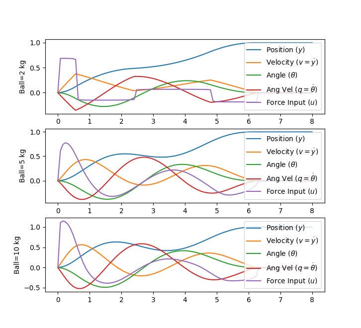
mass = [2,5,10] nm = len(mass) plt.figure()
for j in range(len(mass)):
    m1 = 10
    m2 = mass[j]
    eps = m2/(m1+m2)
    A = np.array([[0,1,0,0],
                 [0,0,eps,0],
                 [0,0,0,1],
                 [0,0,-1,0]])
    B = np.array([[0],
                 [1],
                 [0],
                 [-1]])
    C = np.identity(4)

    m = GEKKO()
    x,y,u = m.state_space(A,B,C,D=None)
    m.time = np.linspace(0,8,101)
    fn = [0 if m.time[i]<6.2 else 1 for i in range(101)]
    final = m.Param(value=fn)
    u[0].status = 1
    m.Obj(final * ((y[0]-1)**2 + y[1]**2 + y[2]**2 + y[3]**2))
    m.options.IMODE = 6
    m.solve()

    plt.subplot(len(mass),1,j+1)
    plt.ylabel(f'Ball={mass[j]} kg')
    plt.plot(m.time,y[0], label = r"Position ($y$)")
    plt.plot(m.time,y[1], label = r"Velocity ($v=\dot y$)")
    plt.plot(m.time,y[2], label = r"Angle ($\theta$)")
    plt.plot(m.time,y[3], label = r"Ang Vel ($q=\dot \theta$)")
    plt.plot(m.time,u[0], label = r"Force Input ($u$)")
    plt.legend(loc=1)
plt.show() (:sourceend:)
Thanks to Derek Prestwich for the state space implementation.
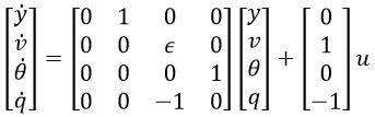
$$\begin{bmatrix} \dot y \\ \dot v \\ \dot \theta \\ \dot q \end{bmatrix}=\begin{bmatrix} 0 & 1 & 0 & 0\\ 0 & 0 & \epsilon & 0\\ 0 & 0 & 0 & 1\\ 0 & 0 & -1 & 0 \end{bmatrix} \begin{bmatrix} y \\ v \\ \theta \\ q \end{bmatrix} + \begin{bmatrix} 0 \\ 1 \\ 0 \\ -1 \end{bmatrix} u$$
(:html:) <iframe width="560" height="315" src="https://www.youtube.com/embed/clMBeJ3FI_g" frameborder="0" allow="autoplay; encrypted-media" allowfullscreen></iframe> (:htmlend:)
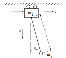
where m1=10 is the mass of the cart, m2=1 is the mass of the item carried, epsilon is m2/(m1+m2), y is the position of the overhead cart, v is the velocity of the overhead cart, theta is the angle of the pendulum relative to the cart, and q is the rate of angle change2.
where m1=10 is the mass of the cart, m2=1 is the mass of the item carried, `\epsilon` is m2/(m1+m2), y is the position of the overhead cart, v is the velocity of the overhead cart, `\theta` is the angle of the pendulum relative to the cart, and q is the rate of angle change2.
ax = fig.add_subplot(111,autoscale_on=False,xlim=(-1.5,0.5),ylim=(-1.2,0.4))
ax = fig.add_subplot(111,autoscale_on=False, xlim=(-1.5,0.5),ylim=(-1.2,0.4))
mass1, = ax.plot([],[],linestyle='None',marker='s',markersize=40,markeredgecolor='k',color='orange',markeredgewidth=2) mass2, = ax.plot([],[],linestyle='None',marker='o',markersize=20,markeredgecolor='k',color='orange',markeredgewidth=2) line, = ax.plot([],[],'o-',color='orange',lw=4,markersize=6,markeredgecolor='k',markerfacecolor='k')
mass1, = ax.plot([],[],linestyle='None',marker='s', markersize=40,markeredgecolor='k', color='orange',markeredgewidth=2) mass2, = ax.plot([],[],linestyle='None',marker='o', markersize=20,markeredgecolor='k', color='orange',markeredgewidth=2) line, = ax.plot([],[],'o-',color='orange',lw=4, markersize=6,markeredgecolor='k', markerfacecolor='k')
ani_a = animation.FuncAnimation(fig, animate, np.arange(1,len(m.time)),
interval=40,blit=False,init_func=init)
ani_a = animation.FuncAnimation(fig, animate, np.arange(1,len(m.time)), interval=40,blit=False,init_func=init)
Thanks to https://www.linkedin.com/in/everton-colling-0161b047/? for the animation code in Python.
Thanks to Everton Colling for the animation code in Python.

(:html:) <iframe width="560" height="315" src="https://www.youtube.com/embed/iTaz8ro-4D4" frameborder="0" allowfullscreen></iframe> (:htmlend:)
(:html:) <iframe width="560" height="315" src="https://www.youtube.com/embed/iTaz8ro-4D4" frameborder="0" allowfullscreen></iframe> (:htmlend:)
(:toggle hide gekko_animate button show="Show GEKKO (Python) and Animation Code":) (:div id=gekko_animate:) (:source lang=python:)
- Contributed by Everton Colling
import matplotlib.animation as animation import numpy as np from gekko import GEKKO
- requires ffmpeg to save mp4 file
- available from https://ffmpeg.zeranoe.com/builds/
- add ffmpeg.exe to path such as C:\ffmpeg\bin\ in
- environment variables
- Defining a model
m = GEKKO()
- Weight of item
m2 = 5
- Defining the time, we will go beyond the 6.2s
- to check if the objective was achieved
m.time = np.linspace(0,8,100)
- Parameters
m1a = m.Param(value=10) m2a = m.Param(value=m2) final = np.zeros(len(m.time)) for i in range(len(m.time)):
    if m.time[i] < 6.2:
        final[i] = 0
    else:
        final[i] = 1
final = m.Param(value=final)
- MV
ua = m.Var(value=0)
- State Variables
theta_a = m.Var(value=0) qa = m.Var(value=0) ya = m.Var(value=-1) va = m.Var(value=0)
- Intermediates
epsilon = m.Intermediate(m2a/(m1a+m2a))
- Defining the State Space Model
m.Equation(ya.dt() == va) m.Equation(va.dt() == epsilon*theta_a + ua) m.Equation(theta_a.dt() == qa) m.Equation(qa.dt() == -theta_a -ua)
- Definine the Objectives
- Make all the state variables be zero at time >= 6.2
m.Obj(final*ya**2) m.Obj(final*va**2) m.Obj(final*theta_a**2) m.Obj(final*qa**2)
- Try to minimize change of MV over all horizon
m.Obj(0.001*ua**2)
m.options.IMODE = 6 #MPC m.solve() #(disp=False)
- Plotting the results
import matplotlib.pyplot as plt plt.figure(figsize=(12,10))
plt.subplot(221) plt.plot(m.time,ua.value,'m',lw=2) plt.legend([r'$u$'],loc=1) plt.ylabel('Force') plt.xlabel('Time') plt.xlim(m.time[0],m.time[-1])
plt.subplot(222) plt.plot(m.time,va.value,'g',lw=2) plt.legend([r'$v$'],loc=1) plt.ylabel('Velocity') plt.xlabel('Time') plt.xlim(m.time[0],m.time[-1])
plt.subplot(223) plt.plot(m.time,ya.value,'r',lw=2) plt.legend([r'$y$'],loc=1) plt.ylabel('Position') plt.xlabel('Time') plt.xlim(m.time[0],m.time[-1])
plt.subplot(224) plt.plot(m.time,theta_a.value,'y',lw=2) plt.plot(m.time,qa.value,'c',lw=2) plt.legend([r'$\theta$',r'$q$'],loc=1) plt.ylabel('Angle') plt.xlabel('Time') plt.xlim(m.time[0],m.time[-1])
plt.rcParams['animation.html'] = 'html5'
x1 = ya.value y1 = np.zeros(len(m.time))
- suppose that l = 1
x2 = 1*np.sin(theta_a.value)+x1 x2b = 1.05*np.sin(theta_a.value)+x1 y2 = -1*np.cos(theta_a.value)+y1 y2b = -1.05*np.cos(theta_a.value)+y1
fig = plt.figure(figsize=(8,6.4)) ax = fig.add_subplot(111,autoscale_on=False,xlim=(-1.5,0.5),ylim=(-1.2,0.4)) ax.set_xlabel('position') ax.get_yaxis().set_visible(False)
crane_rail, = ax.plot([-1.5,0.5],[0.2,0.2],'k-',lw=4) start, = ax.plot([-1,-1],[-1.5,1],'k:',lw=2) objective, = ax.plot([0,0],[-1.5,1],'k:',lw=2) mass1, = ax.plot([],[],linestyle='None',marker='s',markersize=40,markeredgecolor='k',color='orange',markeredgewidth=2) mass2, = ax.plot([],[],linestyle='None',marker='o',markersize=20,markeredgecolor='k',color='orange',markeredgewidth=2) line, = ax.plot([],[],'o-',color='orange',lw=4,markersize=6,markeredgecolor='k',markerfacecolor='k') time_template = 'time = %.1fs' time_text = ax.text(0.05,0.9,'',transform=ax.transAxes) start_text = ax.text(-1.06,-1.1,'start',ha='right') end_text = ax.text(0.06,-1.1,'objective',ha='left')
def init():
    mass1.set_data([],[])
    mass2.set_data([],[])
    line.set_data([],[])
    time_text.set_text('')
    return line, mass1, mass2, time_text
def animate(i):
    mass1.set_data([x1[i]],[y1[i]+0.1])
    mass2.set_data([x2b[i]],[y2b[i]])
    line.set_data([x1[i],x2[i]],[y1[i],y2[i]])
    time_text.set_text(time_template % m.time[i])
    return line, mass1, mass2, time_text
ani_a = animation.FuncAnimation(fig, animate, np.arange(1,len(m.time)),
interval=40,blit=False,init_func=init)
ani_a.save('Pendulum_Control.mp4',fps=30)
plt.show() (:sourceend:)
Thanks to https://www.linkedin.com/in/everton-colling-0161b047/? for the animation code in Python.
(:divend:)
Solution with m2=1
Solution with m2=1
Objective: Design a model predictive controller with a custom objective function that satisfies a specific problem criterion. Simulate and optimize a pendulum system with an adjustable overhead cart. Estimated time: 3 hours.
Objective: Design a model predictive controller for an overhead crane. Meet specific control objectives by tuning the controller and using the state space model of the crane system. Simulate and optimize the pendulum system with an adjustable overhead cart. Estimated time: 2 hours.
plt.subplot(5,1,1) plt.plot(m.time,u.value) plt.ylabel('u') plt.subplot(5,1,2) plt.plot(m.time,v.value) plt.ylabel('velocity') plt.subplot(5,1,3) plt.plot(m.time,y.value) plt.ylabel('y') plt.subplot(5,1,4) plt.plot(m.time,theta.value) plt.ylabel('theta') plt.subplot(5,1,5) plt.plot(m.time,q.value) plt.ylabel('q') plt.xlabel('time')
plt.subplot(4,1,1) plt.plot(m.time,u.value,'r-',LineWidth=2) plt.ylabel('Force') plt.legend(['u'],loc='best') plt.subplot(4,1,2) plt.plot(m.time,v.value,'b--',LineWidth=2) plt.legend(['v'],loc='best') plt.ylabel('Velocity') plt.subplot(4,1,3) plt.plot(m.time,y.value,'g:',LineWidth=2) plt.legend(['y'],loc='best') plt.ylabel('Position') plt.subplot(4,1,4) plt.plot(m.time,theta.value,'m-',LineWidth=2) plt.plot(m.time,q.value,'k.-',LineWidth=2) plt.legend([r'$\theta$','q'],loc='best') plt.ylabel('Angle') plt.xlabel('Time')
(:toggle hide gekko button show="Show GEKKO (Python) Code":) (:div id=gekko:) (:source lang=python:)
- Import packages
import numpy as np from gekko import GEKKO import matplotlib.pyplot as plt
- Build model
- initialize GEKKO model
m = GEKKO()
- time
m.time = np.linspace(0,7,71)
- Parameters
mass1 = m.Param(value=10) mass2 = m.Param(value=1) final = np.zeros(np.size(m.time)) for i in range(np.size(m.time)):
    if m.time[i] >= 6.2:
        final[i] = 1
    else:
        final[i] = 0
final = m.Param(value=final)
- Manipulated variable
u = m.Var(value=0)
- Variables
theta = m.Var(value=0) q = m.Var(value=0)
- Controlled Variable
y = m.Var(value=-1) v = m.Var(value=0)
- Equations
m.Equations([y.dt() == v,
             v.dt() == mass2/(mass1+mass2) * theta + u,
             theta.dt() == q,
             q.dt() == -theta - u])
- Objective
m.Obj(final * (y**2 + v**2 + theta**2 + q**2)) m.Obj(0.001 * u**2)
- Tuning
- global
m.options.IMODE = 6 #control
- Solve
m.solve()
- Plot solution
plt.figure() plt.subplot(5,1,1) plt.plot(m.time,u.value) plt.ylabel('u') plt.subplot(5,1,2) plt.plot(m.time,v.value) plt.ylabel('velocity') plt.subplot(5,1,3) plt.plot(m.time,y.value) plt.ylabel('y') plt.subplot(5,1,4) plt.plot(m.time,theta.value) plt.ylabel('theta') plt.subplot(5,1,5) plt.plot(m.time,q.value) plt.ylabel('q') plt.xlabel('time') plt.show() (:sourceend:) (:divend:)
(:title Control Basics: PID, LQR, MPC:)
(:title Model Predictive Control:)
  m1 = 10
  m2 = 1
The objective of the controller is to adjust the force on the cart to move the pendulum mass to a new final position. Ensure that initial and final velocities and angles of the pendulum are zero. The position of the pendulum mass is initially at -1 and it is desired to move it to the new position of 0 within 6.2 seconds. Demonstrate controller performance with changes in the pendulum position and that the final pendulum mass remains at the final position without oscillation.
The objective of the controller is to adjust the force on the cart to move the pendulum mass to a new final position. Ensure that initial and final velocities and angles of the pendulum are zero. The position of the pendulum mass is initially at -1 and it is desired to move it to the new position of 0 within 6.2 seconds. Demonstrate controller performance with changes in the pendulum position and that the final pendulum mass remains at the final position without oscillation. How does the solution change if the mass of the item carried is increased to m2=5?
where epsilon is m2/(m1+m2), y is the position of the overhead cart, v is the velocity of the overhead cart, theta is the angle of the pendulum relative to the cart, and q is the rate of angle change2.
  m1 = 10
  m2 = 1
where m1=10 is the mass of the cart, m2=1 is the mass of the item carried, epsilon is m2/(m1+m2), y is the position of the overhead cart, v is the velocity of the overhead cart, theta is the angle of the pendulum relative to the cart, and q is the rate of angle change2.
(:html:) <iframe width="560" height="315" src="https://www.youtube.com/embed/iTaz8ro-4D4" frameborder="0" allowfullscreen></iframe> (:htmlend:)
There are many methods to implement control including basic strategies such as a proportional-integral-derivative (PID) controller or more advanced methods such as model predictive techniques. The purpose of this section is to provide a tutorial overview of potential strategies for control of nonlinear systems with linear models. A following section relates methods to implement dynamic control with nonlinear models.
There are many methods to implement control including basic strategies such as a proportional-integral-derivative (PID) controller or more advanced methods such as model predictive techniques. The purpose of this section is to provide a tutorial overview of potential strategies for control of nonlinear systems with linear models.
(:html:) <iframe width="560" height="315" src="https://www.youtube.com/embed/YHAA-uXhI0E?rel=0" frameborder="0" allowfullscreen></iframe> (:htmlend:)
A following section relates methods to implement dynamic control with nonlinear models.
There are many methods to implement control including basic strategies such as a proportional-integral-derivative (PID) controller or more advanced methods such as model predictive techniques. The purpose of this section is to provide a tutorial overview of potential strategies for control of nonlinear systems. A following section relates methods to implement dynamic control with nonlinear models and large-scale constrained optimizers.
There are many methods to implement control including basic strategies such as a proportional-integral-derivative (PID) controller or more advanced methods such as model predictive techniques. The purpose of this section is to provide a tutorial overview of potential strategies for control of nonlinear systems with linear models. A following section relates methods to implement dynamic control with nonlinear models.
Objective: Design a controller to maintain temperature of a chemical reactor. Develop 3 separate controllers (PID, Linear MPC, Nonlinear MPC) in Python or MATLAB/Simulink. Demonstrate controller performance with steps in the set point and disturbance changes. Estimated time: 3 hours.
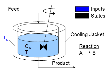
A reactor is used to convert a hazardous chemical A to an acceptable chemical B in waste stream before entering a nearby lake. This particular reactor is dynamically modeled as a Continuously Stirred Tank Reactor (CSTR) with a simplified kinetic mechanism that describes the conversion of reactant A to product B with an irreversible and exothermic reaction. It is desired to maintain the temperature at a constant setpoint that maximizes the destruction of A (highest possible temperature).
Objective: Design a model predictive controller with a custom objective function that satisfies a specific problem criterion. Simulate and optimize a pendulum system with an adjustable overhead cart. Estimated time: 3 hours.
A pendulum is described by the following dynamic equations:
where epsilon is m2/(m1+m2), y is the position of the overhead cart, v is the velocity of the overhead cart, theta is the angle of the pendulum relative to the cart, and q is the rate of angle change2.
The objective of the controller is to adjust the force on the cart to move the pendulum mass to a new final position. Ensure that initial and final velocities and angles of the pendulum are zero. The position of the pendulum mass is initially at -1 and it is desired to move it to the new position of 0 within 6.2 seconds. Demonstrate controller performance with changes in the pendulum position and that the final pendulum mass remains at the final position without oscillation.
- Bryson, A.E., Dynamic Optimization, Addison-Wesley, 1999.
Objective: Design a model predictive controller to maintain temperature of a chemical reactor. Develop a linear, first-order model of the reactor and implement the controller in Python or MATLAB/Simulink. Demonstrate controller performance with steps in the set point and disturbance changes. Estimated time: 3 hours.
Objective: Design a controller to maintain temperature of a chemical reactor. Develop 3 separate controllers (PID, Linear MPC, Nonlinear MPC) in Python or MATLAB/Simulink. Demonstrate controller performance with steps in the set point and disturbance changes. Estimated time: 3 hours.
Objective: Design a model predictive controller to maintain temperature of a chemical reactor. Develop a linear, first-order model of the reactor and implement the model in Python or MATLAB/Simulink. Estimated time: 3 hours.
Objective: Design a model predictive controller to maintain temperature of a chemical reactor. Develop a linear, first-order model of the reactor and implement the controller in Python or MATLAB/Simulink. Demonstrate controller performance with steps in the set point and disturbance changes. Estimated time: 3 hours.
There are many methods to implement control including basic strategies such as a proportional-integral-derivative (PID) controller or more advanced methods such as model predictive techniques. The purpose of this section is to provide a tutorial overview of potential strategies for control of nonlinear systems. A following section relates methods to implement dynamic control with nonlinear models and large-scale constrained optimizers.
There are many methods to implement control including basic strategies such as a proportional-integral-derivative (PID) controller or more advanced methods such as model predictive techniques. The purpose of this section is to provide a tutorial overview of potential strategies for control of nonlinear systems. A following section relates methods to implement dynamic control with nonlinear models and large-scale constrained optimizers.
Exercise
Objective: Design a model predictive controller to maintain temperature of a chemical reactor. Develop a linear, first-order model of the reactor and implement the model in Python or MATLAB/Simulink. Estimated time: 3 hours.
A reactor is used to convert a hazardous chemical A to an acceptable chemical B in waste stream before entering a nearby lake. This particular reactor is dynamically modeled as a Continuously Stirred Tank Reactor (CSTR) with a simplified kinetic mechanism that describes the conversion of reactant A to product B with an irreversible and exothermic reaction. It is desired to maintain the temperature at a constant setpoint that maximizes the destruction of A (highest possible temperature).
Solution
(:title Control Basics: PID, LQR, MPC:) (:keywords Proportional, Integral, Derivative, Linear Quadratic Regulator, Model Predictive Control, simulation, modeling language, differential, algebraic, tutorial:) (:description There are many methods to implement control including basic strategies such as PID or more advanced such as Model Predictive techniques:)
There are many methods to implement control including basic strategies such as a proportional-integral-derivative (PID) controller or more advanced methods such as model predictive techniques. The purpose of this section is to provide a tutorial overview of potential strategies for control of nonlinear systems. A following section relates methods to implement dynamic control with nonlinear models and large-scale constrained optimizers.