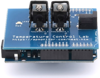
TCLab Stability Analysis
 |  |  |  |  |
|---|
Objective: Determine closed-loop behavior of a P-only controller with the TCLab including oscillatory behavior and stability. Background information on stability analysis may be useful for completing this exercise.


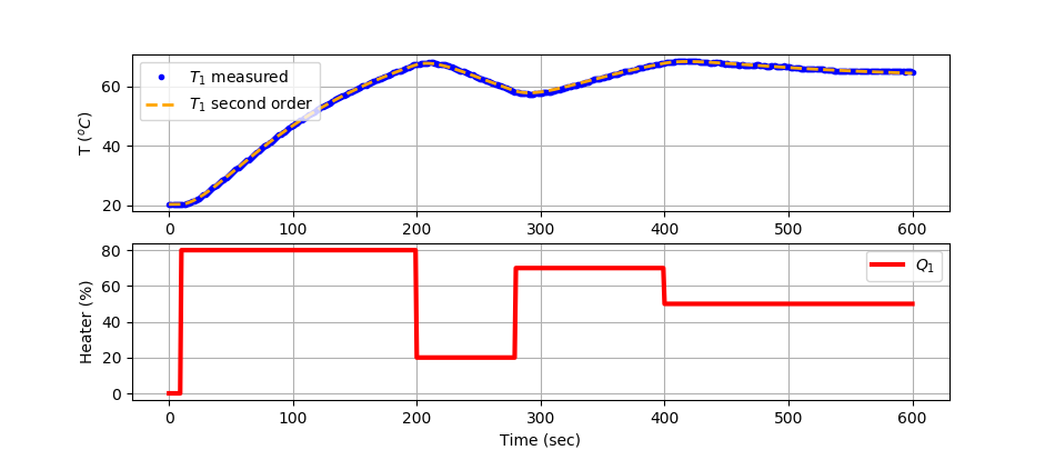
For the temperature control lab, determine a second-order model between heater 1 (Q1) and temperature sensor 1 (TC1).
$$G_p(s) = \frac{T_{C1}(s)}{Q_1(s)} = \frac{K_p}{\tau_s^2\,s^2+2\,\zeta\,\tau_s\,s+1}$$
import matplotlib.pyplot as plt
import pandas as pd
from gekko import GEKKO
import tclab
import time
# Import data
try:
# try to read local data file first
filename = 'data.csv'
data = pd.read_csv(filename)
except:
# heater steps
Q1d = np.zeros(601)
Q1d[10:200] = 80
Q1d[200:280] = 20
Q1d[280:400] = 70
Q1d[400:] = 50
Q2d = np.zeros(601)
try:
# Connect to Arduino
a = tclab.TCLab()
fid = open(filename,'w')
fid.write('Time,Q1,Q2,T1,T2\n')
fid.close()
# run step test (10 min)
for i in range(601):
# set heater values
a.Q1(Q1d[i])
a.Q2(Q2d[i])
print('Time: ' + str(i) + \
' Q1: ' + str(Q1d[i]) + \
' Q2: ' + str(Q2d[i]) + \
' T1: ' + str(a.T1) + \
' T2: ' + str(a.T2))
# wait 1 second
time.sleep(1)
fid = open(filename,'a')
fid.write(str(i)+','+str(Q1d[i])+','+str(Q2d[i])+',' \
+str(a.T1)+','+str(a.T2)+'\n')
fid.close()
# close connection to Arduino
a.close()
except:
filename = 'https://apmonitor.com/pdc/uploads/Main/tclab_data3.txt'
# read either local file or use link if no TCLab
data = pd.read_csv(filename)
# Second order model of TCLab
m = GEKKO()
m.time = data['Time'].values
Kp = m.FV(1.0,lb=0.5,ub=2.0)
taus = m.FV(50,lb=10,ub=200)
zeta = m.FV(1.2,lb=1.1,ub=5)
T0 = data['T1'][0]
Q1 = m.Param(0)
x = m.Var(0); TC1 = m.CV(T0)
m.Equation(x==TC1.dt())
m.Equation((taus**2)*x.dt()+2*zeta*taus*TC1.dt()+(TC1-T0) == Kp*Q1)
m.options.IMODE = 5
m.options.NODES = 2
m.options.EV_TYPE = 2 # Objective type
Kp.STATUS = 1
taus.STATUS = 1
zeta.STATUS = 1
TC1.FSTATUS = 1
Q1.value=data['Q1'].values
TC1.value=data['T1'].values
m.solve(disp=True)
# Parameter values
print('Estimated Parameters')
print('Kp : ' + str(Kp.value[0]))
print('taus: ' + str(taus.value[0]))
print('zeta: ' + str(zeta.value[0]))
# Create plot
plt.figure(figsize=(10,7))
ax=plt.subplot(2,1,1)
ax.grid()
plt.plot(data['Time'],data['T1'],'b.',label=r'$T_1$ measured')
plt.plot(m.time,TC1.value,color='orange',linestyle='--',\
linewidth=2,label=r'$T_1$ second order')
plt.ylabel(r'T ($^oC$)')
plt.legend(loc=2)
ax=plt.subplot(2,1,2)
ax.grid()
plt.plot(data['Time'],data['Q1'],'r-',\
linewidth=3,label=r'$Q_1$')
plt.ylabel('Heater (%)')
plt.xlabel('Time (sec)')
plt.legend(loc='best')
plt.savefig('tclab_2nd_order.png')
plt.show()
With the second-order TCLab model, determine the range of controller gains (Kc) where a P-only controller oscillates and is stable (does not diverge). Traditional stability analysis does not include information about controller output saturation (0-100% heater).
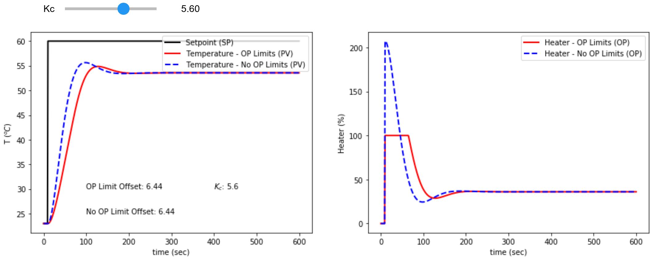
P-Only Simulator
Use the P-Only simulator to test the stability and oscillation predictions. The simulator shows the stability and oscillation of a P-only controller with a TCLab second-order model with `K_p`=0.8473 oC/%, `\tau_s`=51.08 sec, `\zeta`=1.581 sec, and `\theta_p`=0.0 sec. Use the second-order model parameters from your own TCLab device for a more accurate simulation. The controller gain `K_c` is adjusted with a slider to compute the updated temperature response.
%matplotlib inline
import matplotlib.pyplot as plt
from scipy.integrate import odeint
import ipywidgets as wg
from IPython.display import display
n = 601 # time points to plot
tf = 600.0 # final time
# TCLab Second-Order
Kp = 0.8473
taus = 51.08
zeta = 1.581
thetap = 0.0
def process(z,t,u):
x,y = z
dxdt = (1.0/(taus**2)) * (-2.0*zeta*taus*x-(y-23.0) + Kp * u)
dydt = x
return [dxdt,dydt]
def pidPlot(Kc):
t = np.linspace(0,tf,n) # create time vector
P = np.zeros(n) # initialize proportional term
e = np.zeros(n) # initialize error
OP = np.zeros(n) # initialize controller output
PV = np.ones(n)*23.0 # initialize process variable
SP = np.ones(n)*23.0 # initialize setpoint
SP[10:] = 60.0 # step up
z0 = [0,23.0] # initial condition
# loop through all time steps
for i in range(1,n):
# simulate process for one time step
ts = [t[i-1],t[i]] # time interval
z = odeint(process,z0,ts,args=(OP[max(0,i-1-int(thetap))],))
z0 = z[1] # record new initial condition
# calculate new OP with PID
PV[i] = z0[1] # record PV
e[i] = SP[i] - PV[i] # calculate error = SP - PV
dt = t[i] - t[i-1] # calculate time step
P[i] = Kc * e[i] # calculate proportional term
OP[i] = min(100,max(0,P[i])) # calculate new controller output
P = np.zeros(n) # initialize proportional term
e = np.zeros(n) # initialize error
OPu = np.zeros(n) # initialize controller output
PVu = np.ones(n)*23.0 # initialize process variable
SP = np.ones(n)*23.0 # initialize setpoint
SP[10:] = 60.0 # step up
z0 = [0,23.0] # initial condition
# loop through all time steps
for i in range(1,n):
# simulate process for one time step
ts = [t[i-1],t[i]] # time interval
z = odeint(process,z0,ts,args=(OPu[max(0,i-1-int(thetap))],))
z0 = z[1] # record new initial condition
# calculate new OP with PID
PVu[i] = z0[1] # record PV
e[i] = SP[i] - PVu[i] # calculate error = SP - PV
dt = t[i] - t[i-1] # calculate time step
P[i] = Kc * e[i] # calculate proportional term
OPu[i] = P[i] # calculate new controller output
# plot PID response
plt.figure(1,figsize=(15,5))
plt.subplot(1,2,1)
plt.plot(t,SP,'k-',linewidth=2,label='Setpoint (SP)')
plt.plot(t,PV,'r-',linewidth=2,label='Temperature - OP Limits (PV)')
plt.plot(t,PVu,'b--',linewidth=2,label='Temperature - No OP Limits (PV)')
plt.ylabel(r'T $(^oC)$')
plt.text(100,30,'OP Limit Offset: ' + str(np.round(SP[-1]-PVu[-1],2)))
M = SP[-1]-SP[0]
pred_offset = M*(1-Kp*Kc/(1+Kp*Kc))
plt.text(100,25,'No OP Limit Offset: ' + str(np.round(pred_offset,2)))
plt.text(400,30,r'$K_c$: ' + str(np.round(Kc,1)))
plt.legend(loc=1)
plt.xlabel('time (sec)')
plt.subplot(1,2,2)
plt.plot(t,OP,'r-',linewidth=2,label='Heater - OP Limits (OP)')
plt.plot(t,OPu,'b--',linewidth=2,label='Heater - No OP Limits (OP)')
plt.ylabel('Heater (%)')
plt.legend(loc='best')
plt.xlabel('time (sec)')
Kc_slide = wg.FloatSlider(value=2.0,min=-2.0,max=10.0,step=0.1)
wg.interact(pidPlot, Kc=Kc_slide)
print('P-only Simulator with and without OP Limits: Adjust Kc')
Solution
The second-order parameter regression gives the following parameters:
$$K_p= 0.8473$$
$$\tau_s= 51.08$$
$$\zeta = 1.581$$
$$G_p(s)=\frac{K_p}{\tau_s^2\,s^2+2\,\zeta\,\tau_s\,s+1}$$
The controller stability range is analyzed with a Routh Array and Root Locus plot. The Root Locus plot also shows where the controller begins to oscillate.
Routh Array
The closed-loop transfer function with a P-only controller gain `K_c` is:
$$G_{cl}(s)=\frac{T_{C1}(s)}{T_{SP}(s)}=\frac{K_c\,G_p(s)}{1+K_c\,G_p(s)}=\frac{\frac{K_c\,K_p}{\tau_s^2\,s^2+2\,\zeta\,\tau_s\,s+1}}{1+\frac{K_c\,K_p}{\tau_s^2\,s^2+2\,\zeta\,\tau_s\,s+1}}=\frac{K_c\,K_p}{\tau_s^2\,s^2+2\,\zeta\,\tau_s\,s+1+K_c\,K_p}$$
The coefficients of the denominator are analyzed to determine the stability range.
| `a_n=\tau_s^2` | `a_{n-2}=1+K_c\,K_p` |
| `a_{n-1}=2 \zeta \tau_s` | `a_{n-3}=0` |
| `b_{1}=\frac{(2 \zeta \tau_s)(1+K_c K_p)}{2 \zeta \tau_s}=1+K_c K_p` | `b_{2}=0` |
| `c_{1}=0` | 0 |
The leading edge cannot change signs for the system to be stable. Therefore, the following conditions must be met:
$$a_n=\tau_s^2=2609 > 0$$
$$a_{n-1}=2\,\zeta\,\tau_s=161.4 > 0$$
$$b_{1}=1+K_c\,K_p > 0$$
$$c_{1}=0 > 0$$
The positive constraint on `b_1` leads to `K_c`>`-\frac{1}{K_p}`. Therefore the following range is acceptable for the controller stability.
$$K_c > -1.1803$$
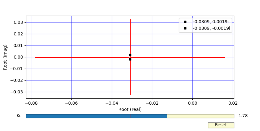
Root Locus Plot
One of the real portion of the roots becomes positive when `K_c`<-1.19. There is no positive value of the controller gain that leads to an unstable system. This implies that the only way to make a second-order system unstable is to incorrectly specify the controller as a Direct acting controller with a value at least equal to the inverse of the process gain. The unstable controller does not have imaginary roots so the response is expect to go to `+\infty` or `-\infty` without oscillation.
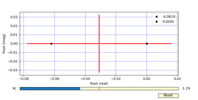
There are imaginary roots and oscillation when `K_c`>1.78. The real portion of the roots are negative so the system is stable and converges but not necessarily to the new set point.
import math
import numpy as np
import matplotlib.pyplot as plt
from matplotlib.widgets import Slider, Button, RadioButtons
Kp = 0.84726
taus = 51.0800
zeta = 1.58068
# open loop
num = [Kp]
den = [taus**2,2*zeta*taus,1]
# demoninator of the closed loop
# Gcl = direct/(1+loop)
def dcl(K):
return [taus**2,2*zeta*taus,1.0+K*Kp]
# root locus plot
n = 10000 # number of points to plot
nr = len(den)-1 # number of roots
rs = np.zeros((n,2*nr)) # store results
Kc1 = -5.0
Kc2 = 5.0
Kc = np.linspace(Kc1,Kc2,n) # Kc values
for i in range(n): # cycle through n times
roots = np.roots(dcl(Kc[i]))
for j in range(nr): # store roots
rs[i,j] = roots[j].real # store real
rs[i,j+nr] = roots[j].imag # store imaginary
# create the image
fig, ax = plt.subplots()
plt.subplots_adjust(left=0.10, bottom=0.25)
ls = []
for i in range(nr):
plt.plot(rs[:,i],rs[:,i+nr],'r.',markersize=2)
# this handle is required to update the plot
if math.isclose(rs[0,i+nr],0.0):
lbl = f'{rs[0,i]:0.4f}'
else:
lbl = f'{rs[0,i]:0.4f}, {rs[0,i+nr]:0.4f}i'
l, = plt.plot(rs[0,i],rs[0,i+nr], 'ks', markersize=5,label=lbl)
ls.append(l)
leg = plt.legend(loc='best')
plt.xlabel('Root (real)')
plt.ylabel('Root (imag)')
plt.grid(b=True, which='major', color='b', linestyle='-',alpha=0.5)
plt.grid(b=True, which='minor', color='r', linestyle='--',alpha=0.5)
# slider creation
axcolor = 'lightgoldenrodyellow'
axKc = plt.axes([0.10, 0.1, 0.80, 0.03], facecolor=axcolor)
sKc = Slider(axKc, 'Kc', Kc1, Kc2, valinit=0, valstep=0.01)
def update(val):
Kc_val= sKc.val
indx = (np.abs(Kc-Kc_val)).argmin()
for i in range(nr):
ls[i].set_ydata(rs[indx,i+nr])
ls[i].set_xdata(rs[indx,i])
if math.isclose(rs[indx,i+nr],0.0):
lbl = f'{rs[indx,i]:0.4f}'
else:
lbl = f'{rs[indx,i]:0.4f}, {rs[indx,i+nr]:0.4f}i'
leg.texts[i].set_text(lbl)
fig.canvas.draw_idle()
sKc.on_changed(update)
resetax = plt.axes([0.8, 0.025, 0.1, 0.04])
button = Button(resetax, 'Reset', color=axcolor, hovercolor='0.975')
def reset(event):
sKc.reset()
button.on_clicked(reset)
plt.show()
Extra: Calculate Offset
If there were a set point change of +M with `T_{SP}(s)=\frac{M}{s}` then the temperature response is predicted to increase:
$$T_{C1,\infty} = \lim_{s \to 0} s \, T_{C1}(s) = \lim_{s \to 0} s \, G_{cl}(s)\frac{M}{s} = \frac{M\,K_p\,K_c}{1+K_p\,K_c}$$
This gives an offset of:
$$\mathrm{Offset} = T_{SP} - T_{C1,\infty} = M \left(1 - \frac{K_p\,K_c}{1+K_p\,K_c} \right)$$