Dynamics and Control

Objective: Demonstrate the use of several methods to determine system characteristics including oscillatory behavior and stability. Background information on stability analysis may be useful for completing these exercises.

Problem 1

Determine characteristics of the following systems including:

• Diverges or Converges
• Oscillatory or Smooth
• The final value of a step response as `y(t \to \infty)` with input `U(s)=\frac{1}{s}`
• Plot of the step response `y(t)` to verify the solution.

Part A

$$G(s) = \frac{Y(s)}{U(s)} = \frac{4}{(s-1)^2 (s+2)(s+3)}$$

Part B

$$G(s) = \frac{Y(s)}{U(s)} = \frac{s^2-s+2}{(s+1)^{10} (s^2+s+1)}$$

Part C

$$G(s) = \frac{Y(s)}{U(s)} = \frac{s-3}{(s-3) (s+1) (s^2+s+1)}$$

Problem 2

Determine the values of `K_c` that keep the closed loop system response stable with the following open loop transfer function.

$$G_{OL} = \frac{-2 \, K_c}{\left(s^2+s+1\right) \left(s+1\right)^2}$$

Use the Routh Array method to determine the upper and lower limits for controller stability. Transfer function simulation, root locus, and Bode plot code is available to confirm the solution with other stability analysis methods. To see the plots, run Simulate Problem 2.

import numpy as np
from scipy import signal
import matplotlib.pyplot as plt

# open loop
num = [-2.0]
den = [1.0,3.0,4.0,3.0,1.0]
sys = signal.TransferFunction(num, den)
t1,y1 = signal.step(sys)

plt.figure(1)
plt.plot(t1,y1,'k-')
plt.legend(['Open Loop'],loc='best')

# closed loop
plt.figure(2)
n = 6
Kc = np.linspace(-1.1,0.6,n)  # Kc values
t = np.linspace(0,100,1000) # time values
for i in range(n):
    num = [-2.0*Kc[i]]
    den = [1.0,3.0,4.0,3.0,1.0-2.0*Kc[i]]
    sys2 = signal.TransferFunction(num, den)
    t2,y2 = signal.step(sys2,T=t)
    plt.plot(t2,y2,label='Kc='+str(Kc[i]))
plt.ylim([-2,3])
plt.legend(loc='best')
plt.xlabel('Time')

# root locus plot
import numpy.polynomial.polynomial as poly
n = 1000  # number of points to plot
nr = 4    # number of roots
rs = np.zeros((n,2*nr))   # store results
Kc1 = -2.0
Kc2 = 1.0
Kc = np.linspace(Kc1,Kc2,n)  # Kc values
for i in range(n):        # cycle through n times
    den = [1.0,3.0,4.0,3.0,1.0-2.0*Kc[i]]
    roots = poly.polyroots(den) # find roots
    for j in range(nr):   # store roots
        rs[i,j] = roots[j].real # store real
        rs[i,j+nr] = roots[j].imag # store imaginary

plt.figure(3)
plt.xlabel('Root (real)')
plt.ylabel('Root (imag)')
plt.grid(b=True, which='major', color='b', linestyle='-')
plt.grid(b=True, which='minor', color='r', linestyle='--')
for i in range(nr):
    plt.plot(rs[:,i],rs[:,i+nr],'.')
plt.xlim([-1.5,0.5])
plt.ylim([-1.2,1.2])

plt.figure(4)
plt.subplot(2,1,1)
for i in range(nr):
    plt.plot(Kc,rs[:,i],'.')
plt.ylabel('Root (real part)')
plt.xlabel('Controller Gain (Kc)')
plt.xlim([Kc1,Kc2])
plt.ylim([-1,1])

plt.subplot(2,1,2)
for i in range(nr):
    plt.plot(Kc,rs[:,i+nr],'.')
plt.ylabel('Root (imag part)')
plt.xlabel('Controller Gain (Kc)')
plt.xlim([Kc1,Kc2])
plt.ylim([-2,2])


# bode plot
w,mag,phase = signal.bode(sys)
plt.figure(5)
plt.subplot(2,1,1)
plt.semilogx(w,mag,'k-',linewidth=3)
plt.grid(b=True, which='major', color='b', linestyle='-')
plt.grid(b=True, which='minor', color='r', linestyle='--')
plt.ylabel('Magnitude')

plt.subplot(2,1,2)
plt.semilogx(w,phase,'k-',linewidth=3)
plt.grid(b=True, which='major', color='b', linestyle='-')
plt.grid(b=True, which='minor', color='r', linestyle='--')
plt.ylabel('Phase')
plt.xlabel('Frequency')

plt.show()

[$[Get Code]]

Problem 3

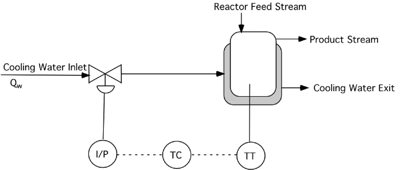
Cooling water flows through a jacket to control the temperature of a reactor, as shown below. The transfer function relating the reactor temperature T to the flow rate of cooling water through the jacket (`Q_w`) is

$$\frac{T(s)}{Q_w(s)} = \frac{-0.7}{(s+1)(2s-1)} \frac{^oF}{gpm}$$

where the time constants are in minutes. The valve on the cooling water inlet fails in the open position (air-to-close), and passes 360 gpm of water when completely open. You may assume that the pressure drop across the valve is constant, that valve dynamics are negligible, and that the valve is linear. The temperature transmitter has a range of 200-400 degF and requires about 0.5 minutes for a reading to reach its final value (`3 \tau` to `5 \tau`). The output from the transmitter is a 4-20 mA signal to the reverse-acting controller. The proportional-only controller outputs a current signal, which is converted to pressure in a standard I/P transducer (4-20 mA, 3-15 psig). Sketch a block diagram for the system and determine the transfer function for each of the blocks, including units.

The process is unstable, but stable operation can be achieved with the feedback control loop shown and a proportional-only controller. What range of values of Kc (if any) will make this process stable?

Problem 1 Solution

Problem 1 - Simulate Step Responses

import numpy as np
from scipy import signal
import matplotlib.pyplot as plt

name = 'Problem 1A'
num = [4.0]
p1 = np.poly1d([1,-1])
p2 = np.poly1d([1,2])
p3 = np.poly1d([1,3])
den = p1*p2*p3
sys = signal.TransferFunction(num,den)
t,y = signal.step(sys)
plt.figure(1)
plt.plot(t,y,'k-',label=name)
plt.legend(loc='best')

name = 'Problem 1B'
num = [1,-1,2]
p1 = [1,1]
p2 = [1,1,1]
den = p1
t = np.linspace(0,50,1000)
for i in range(9):
    den = np.convolve(den,p1)
den = np.convolve(den,p2)
print(den)
sys = signal.TransferFunction(num,den)
t,y = signal.step(sys,T=t)
plt.figure(2)
plt.plot(t,y,'k-',label=name)
plt.legend(loc='best')

name = 'Problem 1C'
num = [1]
p1 = np.poly1d([1,1])
p2 = np.poly1d([1,1,1])
den = p1*p2
print(den)
sys = signal.TransferFunction(num,den)
t,y = signal.step(sys,T=t)
plt.figure(3)
plt.plot(t,y,'k-',label=name)
plt.legend(loc='best')
plt.show()

[$[Get Code]]

Problem 2 Solution

Problem 3 Solution

The stability limits are determined with a Root Locus plot or with a Routh array method.

import numpy as np
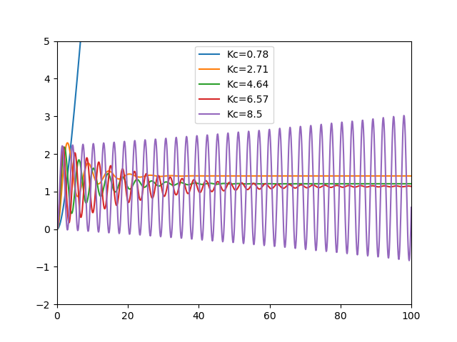
from scipy import signal
import matplotlib.pyplot as plt

a = 0.08*0.75*30*0.7
n = 5
Kc = np.linspace(0.78,8.5,n)
tm = np.linspace(0,100,1000)
for Kci in Kc:
    num = [a*0.1*Kci,a*Kci]
    den = [0.2,2.1,0.9,-1+1.26*Kci]
    sys = signal.TransferFunction(num,den)
    t,y = signal.step(sys,T=tm)
    plt.plot(t,y,label='Kc='+str(Kci))
plt.legend(loc='best')
plt.xlim([0,100])
plt.ylim([-2,5])
plt.show()

[$[Get Code]]