TCLab PID with Feedforward
 |  |  |  |
|---|
Objective: Add a feedforward trim to a PID controller on heater 1 to reject temperature disturbances from heater 2.
Test the performance with a temperature 1 setpoint change from ambient temperature to 40oC at 10 sec and adjust heater 2 from 0% to 100% at 200 sec and heater 2 back to 0% at 400 sec. The test should continue for 600 sec (10 min). Select a feedforward gain to reject the temperature 2 disturbance.
Feedforward control is an additional term in the PID equation that adds or removes control action `Q_1(t)` based on a measured disturbance `T_2`. Feedforward trim is added to a PID controller with the addition of a final term where `T_2` is the measured disturbance.
$$e(t) = T_{sp}-T_1$$
$$Q_1(t) = Q_{1,bias} + K_c \, e(t) + \frac{K_c}{\tau_I}\int_0^t e(t)dt - K_c \tau_D \frac{d(T_1)}{dt} + \color{blue}{K_{ff}\,T'_2}$$
For this exercise, set the feedforward control gain to a ratio of the disturbance and process gains.
$$K_{ff} = -\frac{K_d}{K_p}$$
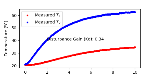
Determine the disturbance gain `K_d=\frac{\Delta T_1}{\Delta T_2}` by performing a step test with heater 2 to 100% and observe the steady-state change in `T_1` and `T_2`.
import matplotlib.pyplot as plt
import tclab
import time
n = 600 # Number of second time points (10 min)
tm = np.linspace(0,n,n+1) # Time values
# data
lab = tclab.TCLab()
T1 = [lab.T1]
T2 = [lab.T2]
lab.Q2(100)
for i in range(n):
time.sleep(1)
print(lab.T1,lab.T2)
T1.append(lab.T1)
T2.append(lab.T2)
lab.close()
# Disturbance Gain
Kd = (T1[-1]-T1[0]) / (T2[-1]-T2[0])
# Plot results
plt.figure(1)
plt.plot(tm/60.0,T1,'r.',label=r'Measured $T_1$')
plt.plot(tm/60.0,T2,'b.',label=r'Measured $T_2$')
plt.text(3,40,'Disturbance Gain (Kd): '+str(round(Kd,2)))
plt.ylabel(r'Temperature ($^o$C)')
plt.xlabel('Time (min)')
plt.legend()
plt.savefig('Disturbance_gain.png')
plt.show()
TCLab PID with Feedforward Simulator
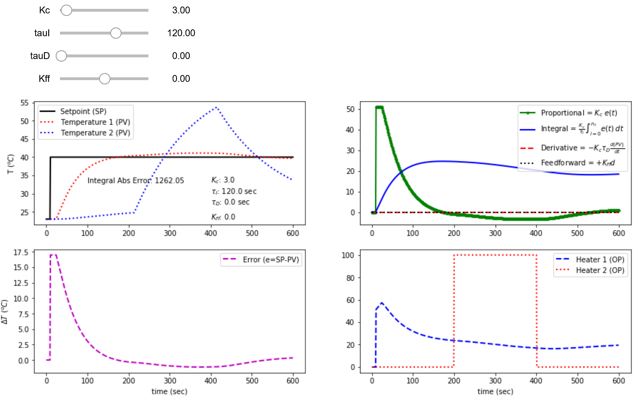
A simulator evaluates the feedforward tuning before implementation on the TCLab. Use the PID with feedforward simulator to find acceptable control performance that best rejects the disturbance.


%matplotlib inline
import matplotlib.pyplot as plt
from scipy.integrate import odeint
import ipywidgets as wg
from IPython.display import display
n = 601 # time points to plot
tf = 600.0 # final time
# TCLab FOPDT
Kp = 0.9
Kd = 0.34
taup = 175.0
thetap = 15.0
y0 = [23.0,23.0]
def process(y,t,u1,u2):
y1,y2 = y
dy1dt = (1.0/taup) * (-(y1-y0[0]) + Kp * u1 + Kd * (y2-y1))
dy2dt = (1.0/taup) * (-(y2-y0[1]) + (Kp/2.0) * u2 + Kd * (y1-y2))
return [dy1dt,dy2dt]
def pidPlot(Kc,tauI,tauD,Kff):
y0 = [23.0,23.0]
t = np.linspace(0,tf,n) # create time vector
P = np.zeros(n) # initialize proportional term
I = np.zeros(n) # initialize integral term
D = np.zeros(n) # initialize derivative term
FF = np.zeros(n) # initialize feedforward term
e = np.zeros(n) # initialize error
OP1 = np.zeros(n) # initialize controller output
OP2 = np.zeros(n) # initialize disturbance
OP2[200:401] = 100 # step up in heater 2
PV1 = np.ones(n)*y0[0] # initialize process variable
PV2 = np.ones(n)*y0[1] # initialize process variable
SP = np.ones(n)*y0[0] # initialize setpoint
SP[10:] = 40.0 # step up
iae = 0.0
# loop through all time steps
for i in range(1,n):
# simulate process for one time step
ts = [t[i-1],t[i]] # time interval
heaters = (OP1[max(0,i-int(thetap))],OP2[max(0,i-int(thetap))])
y = odeint(process,y0,ts,args=heaters)
y0 = y[1] # record new initial condition
# calculate new OP with PID
PV1[i] = y[1][0] # record T1 PV
PV2[i] = y[1][1] # record T2 PV
iae += np.abs(SP[i]-PV1[i])
e[i] = SP[i] - PV1[i] # calculate error = SP - PV
dt = t[i] - t[i-1] # calculate time step
P[i] = Kc * e[i] # calculate proportional term
I[i] = I[i-1] + (Kc/tauI) * e[i] * dt # calculate integral term
D[i] = -Kc * tauD * (PV1[i]-PV1[i-1])/dt # calculate derivative
FF[i] = Kff * (PV2[i]-PV1[i])
OP1[i] = P[i] + I[i] + D[i] + FF[i] # calculate new output
if OP1[i]>=100:
OP1[i] = 100.0
I[i] = I[i-1] # reset integral
if OP1[i]<=0:
OP1[i] = 0.0
I[i] = I[i-1] # reset integral
# plot PID response
plt.figure(1,figsize=(15,7))
plt.subplot(2,2,1)
plt.plot(t,SP,'k-',linewidth=2,label='Setpoint (SP)')
plt.plot(t,PV1,'r:',linewidth=2,label='Temperature 1 (PV)')
plt.plot(t,PV2,'b:',linewidth=2,label='Temperature 2 (PV)')
plt.ylabel(r'T $(^oC)$')
plt.text(100,33,'Integral Abs Error: ' + str(np.round(iae,2)))
plt.text(400,33,r'$K_c$: ' + str(np.round(Kc,0)))
plt.text(400,30,r'$\tau_I$: ' + str(np.round(tauI,0)) + ' sec')
plt.text(400,27,r'$\tau_D$: ' + str(np.round(tauD,0)) + ' sec')
plt.text(400,23,r'$K_{ff}$: ' + str(np.round(Kff,0)))
plt.legend(loc=2)
plt.subplot(2,2,2)
plt.plot(t,P,'g.-',linewidth=2,label=r'Proportional = $K_c \; e(t)$')
plt.plot(t,I,'b-',linewidth=2,label=r'Integral = ' + \
r'$\frac{K_c}{\tau_I} \int_{i=0}^{n_t} e(t) \; dt $')
plt.plot(t,D,'r--',linewidth=2,label=r'Derivative = ' + \
r'$-K_c \tau_D \frac{d(PV)}{dt}$')
plt.plot(t,FF,'k:',linewidth=2,label=r'Feedforward = ' + \
r'$+K_{ff} d$')
plt.legend(loc='best')
plt.subplot(2,2,3)
plt.plot(t,e,'m--',linewidth=2,label='Error (e=SP-PV)')
plt.ylabel(r'$\Delta T$ $(^oC)$')
plt.legend(loc='best')
plt.xlabel('time (sec)')
plt.subplot(2,2,4)
plt.plot(t,OP1,'b--',linewidth=2,label='Heater 1 (OP)')
plt.plot(t,OP2,'r:',linewidth=2,label='Heater 2 (OP)')
plt.legend(loc='best')
plt.xlabel('time (sec)')
Kc_slide = wg.FloatSlider(value=3.0,min=0.0,max=50.0,step=1.0)
tauI_slide = wg.FloatSlider(value=120.0,min=20.0,max=180.0,step=5.0)
tauD_slide = wg.FloatSlider(value=0.0,min=0.0,max=20.0,step=1.0)
Kff_slide = wg.FloatSlider(value=0.0,min=-0.5,max=0.5,step=0.1)
wg.interact(pidPlot, Kc=Kc_slide, tauI=tauI_slide, tauD=tauD_slide,Kff=Kff_slide)
print('PID with Feedforward Simulator: Adjust Kc, tauI, tauD, and Kff ' + \
'to achieve lowest Integral Abs Error')
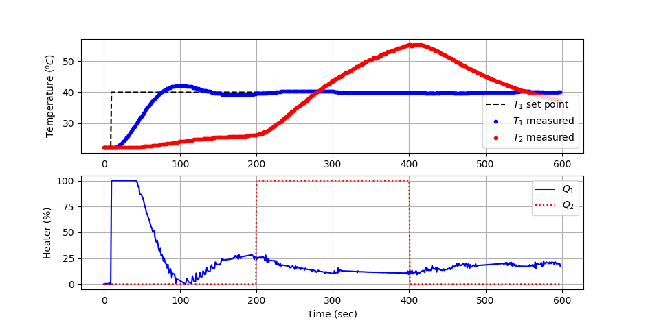
TCLab PID Control Test Script
The TCLab PID control validation script implements the best PID tuning values and calculates the integral absolute error with a sequence of setpoint changes from 23oC initially to 40oC at 10 sec. The heater 2 disturbance (0-100%) between 200-400 sec is also implemented. Update the PID tuning parameters and feedforward gain before running the script.
Kc = 5.0
tauI = 120.0 # sec
tauD = 2.0 # sec
Kff = 0.0
import numpy as np
import time
import matplotlib.pyplot as plt
from scipy.integrate import odeint
#-----------------------------------------
# PID controller performance for the TCLab
#-----------------------------------------
# PID Parameters
Kc = 5.0
tauI = 120.0 # sec
tauD = 2.0 # sec
Kff =
#-----------------------------------------
# PID Controller with Feedforward
#-----------------------------------------
# inputs ---------------------------------
# sp = setpoint
# pv = current temperature
# pv_last = prior temperature
# ierr = integral error
# dt = time increment between measurements
# outputs --------------------------------
# op = output of the PID controller
# P = proportional contribution
# I = integral contribution
# D = derivative contribution
def pid(sp,pv,pv_last,ierr,dt,d):
# Parameters in terms of PID coefficients
KP = Kc
KI = Kc/tauI
KD = Kc*tauD
# ubias for controller (initial heater)
op0 = 0
# upper and lower bounds on heater level
ophi = 100
oplo = 0
# calculate the error
error = sp-pv
# calculate the integral error
ierr = ierr + KI * error * dt
# calculate the measurement derivative
dpv = (pv - pv_last) / dt
# calculate the PID output
P = KP * error
I = ierr
D = -KD * dpv
FF = Kff * d
op = op0 + P + I + D + FF
# implement anti-reset windup
if op < oplo or op > ophi:
I = I - KI * error * dt
# clip output
op = max(oplo,min(ophi,op))
# return the controller output and PID terms
return [op,P,I,D,FF]
# save txt file with data and set point
# t = time
# u1,u2 = heaters
# y1,y2 = tempeatures
# sp1,sp2 = setpoints
def save_txt(t, u1, u2, y1, y2, sp1, sp2):
data = np.vstack((t, u1, u2, y1, y2, sp1, sp2)) # vertical stack
data = data.T # transpose data
top = ('Time,Q1,Q2,T1,T2,TSP1,TSP2')
np.savetxt('validate.txt', data, delimiter=',',\
header=top, comments='')
# Connect to Arduino
a = tclab.TCLab()
# Turn LED on
print('LED On')
a.LED(100)
# Run time in minutes
run_time = 10.0
# Number of cycles
loops = int(60.0*run_time)
tm = np.zeros(loops)
# Temperature
# set point (degC)
Tsp1 = np.ones(loops) * a.T1
# Heater set point steps
Tsp1[10:] = 40.0
T1 = np.ones(loops) * a.T1 # measured T (degC)
error_sp = np.zeros(loops)
Tsp2 = np.ones(loops) * a.T2 # set point (degC)
T2 = np.ones(loops) * a.T2 # measured T (degC)
# impulse tests (0 - 100%)
Q1 = np.ones(loops) * 0.0
Q2 = np.ones(loops) * 0.0
Q2[200:401] = 100.0
print('Running Main Loop. Ctrl-C to end.')
print(' Time SP PV Q1 = P + I + D + FF IAE')
print(('{:6.1f} {:6.2f} {:6.2f} ' + \
'{:6.2f} {:6.2f} {:6.2f} {:6.2f} {:6.2f} {:6.2f}').format( \
tm[0],Tsp1[0],T1[0], \
Q1[0],0.0,0.0,0.0,0.0,0.0))
# Main Loop
start_time = time.time()
prev_time = start_time
dt_error = 0.0
# Integral error
ierr = 0.0
# Integral absolute error
iae = 0.0
plt.figure(figsize=(10,7))
plt.ion()
plt.show()
try:
for i in range(1,loops):
# Sleep time
sleep_max = 1.0
sleep = sleep_max - (time.time() - prev_time) - dt_error
if sleep>=1e-4:
time.sleep(sleep-1e-4)
else:
print('exceeded max cycle time by ' + str(abs(sleep)) + ' sec')
time.sleep(1e-4)
# Record time and change in time
t = time.time()
dt = t - prev_time
if (sleep>=1e-4):
dt_error = dt-1.0+0.009
else:
dt_error = 0.0
prev_time = t
tm[i] = t - start_time
# Read temperatures in Kelvin
T1[i] = a.T1
T2[i] = a.T2
# Disturbance
d = T2[i] - 23.0
# Integral absolute error
iae += np.abs(Tsp1[i]-T1[i])
# Calculate PID output
[Q1[i],P,ierr,D,FF] = pid(Tsp1[i],T1[i],T1[i-1],ierr,dt,d)
# Write output (0-100)
a.Q1(Q1[i])
a.Q2(Q2[i])
# Print line of data
print(('{:6.1f} {:6.2f} {:6.2f} ' + \
'{:6.2f} {:6.2f} {:6.2f} {:6.2f} {:6.2f} {:6.2f}').format( \
tm[i],Tsp1[i],T1[i], \
Q1[i],P,ierr,D,FF,iae))
# Update plot
plt.clf()
# Plot
ax=plt.subplot(2,1,1)
ax.grid()
plt.plot(tm[0:i],Tsp1[0:i],'k--',label=r'$T_1$ set point')
plt.plot(tm[0:i],T1[0:i],'b.',label=r'$T_1$ measured')
plt.plot(tm[0:i],T2[0:i],'r.',label=r'$T_2$ measured')
plt.ylabel(r'Temperature ($^oC$)')
plt.legend(loc=4)
ax=plt.subplot(2,1,2)
ax.grid()
plt.plot(tm[0:i],Q1[0:i],'b-',label=r'$Q_1$')
plt.plot(tm[0:i],Q2[0:i],'r:',label=r'$Q_2$')
plt.ylabel('Heater (%)')
plt.legend(loc=1)
plt.xlabel('Time (sec)')
plt.draw()
plt.pause(0.05)
# Turn off heaters
a.Q1(0)
a.Q2(0)
a.close()
# Save text file
save_txt(tm[0:i],Q1[0:i],Q2[0:i],T1[0:i],T2[0:i],Tsp1[0:i],Tsp2[0:i])
# Save figure
plt.savefig('PID_Control.png')
# Allow user to end loop with Ctrl-C
except KeyboardInterrupt:
# Disconnect from Arduino
a.Q1(0)
a.Q2(0)
print('Shutting down')
a.close()
save_txt(tm[0:i],Q1[0:i],Q2[0:i],T1[0:i],T2[0:i],Tsp1[0:i],Tsp2[0:i])
plt.savefig('PID_Control.png')
# Make sure serial connection closes with an error
except:
# Disconnect from Arduino
a.Q1(0)
a.Q2(0)
print('Error: Shutting down')
a.close()
save_txt(tm[0:i],Q1[0:i],Q2[0:i],T1[0:i],T2[0:i],Tsp1[0:i],Tsp2[0:i])
plt.savefig('PID_Control.png')
raise
Solution
The first step is to determine `K_d`, the disturbance gain. Using the script above and turning on heater 2 to 100% for 10 minutes, temperature 2 rises above 60oC while temperature 1 settles at about 35oC. The gain of the adjacent heater temperature is 0.34, meaning that a 1oC rise in one heater leads to a 0.34oC rise in the other heater. This is due to convective and radiative heater transfer between the two heaters.
The feedforward control gain is set to a ratio of the disturbance and process gains.
$$K_{ff} = -\frac{K_d}{K_p} = -\frac{0.34}{0.9} = -0.38$$
This is implemented in the PID equation with an additional term as shown in blue.
$$Q_1(t) = K_c \, e(t) + \frac{K_c}{\tau_I}\int_0^t e(t)dt - K_c \tau_D \frac{d(T_1)}{dt} + \color{blue}{K_{ff}\,\left(T_2-23\right)}$$
Kc = 10.0
tauI = 50.0 # sec
tauD = 2.0 # sec
Kff = -0.38
What to Turn In
- Disturbance Gain Report: include `K_d = \frac{\Delta T_1}{\Delta T_2}` from the heater 2 step test with a short explanation and supporting plot.
- Feedforward Design: show the calculated `K_{ff} = -\frac{K_d}{K_p}` and briefly explain how this value was determined.
- Simulator Results: plots from the PID with feedforward simulator showing:
- Baseline PID response (no feedforward)
- Improved response with feedforward term
- Annotated values of `K_c`, `\tau_I`, `\tau_D`, `K_{ff}`
- TCLab Validation Plot: temperature and heater responses (T1, T2, Q1, Q2) for the 600-second test.
- Performance Summary: report the Integral Absolute Error (IAE) and discuss feedforward effectiveness in rejecting the heater 2 disturbance.
- Final Tuning Table: best `K_c`, `\tau_I`, `\tau_D`, `K_{ff}` used for the TCLab test.