Objective: Compare an analytic solution of a FOPDT model with an impulse response of the TCLab.

Perform a two minute impulse test with heater 1 to 70% starting at 10 seconds for 1 minute (between 10 and 70 seconds) and continue until 120 seconds.

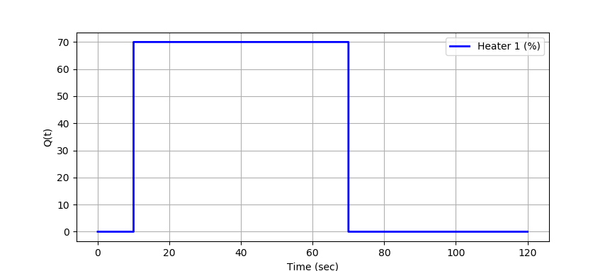
Create a plot of the temperature response over 2 minutes that shows the heater level (%), measured temperature (^oC), and predicted temperature (^oC). Instead of using an ODE solver, derive an analytical solution and simulate a first order plus dead time (FOPDT) model. The FOPDT model is:

$$\tau_p \frac{dT'}{dt} = -T' + K_p \, Q'\left(t-\theta_p\right)$$

where `T'=T-T_{ss}` and `Q'=Q-Q_{ss}` are deviation variables with steady-state initial conditions `T_{ss}=T_{ambient}` and `Q_{ss}=0 \%`. Use the following script to generate a plot (Impulse_Response.png) and data file (Impulse_Response.csv).

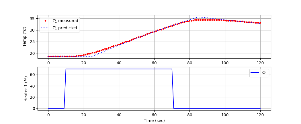
Use values of `K_p`=0.9^oC/%, `\tau_p`=190 sec, and `\theta_p`=15 sec to compute the analytic solution.

Solution

Apply the Laplace transform to each of the terms in the FOPDT equation. Because the Laplace transform is a linear operator, each term can be transformed separately. Because T'(t) is a deviation variable, the initial condition at the initial time is T'(0)=0.

$$\mathcal{L}\left(\tau_p \frac{dT'(t)}{dt}\right) = \tau_p \left(s \, T(s) - T'(0)\right) = \tau_p s \, T(s)$$

$$\mathcal{L}\left(-T'(t)\right) = -T(s)$$

$$\mathcal{L}\left(K_p \, Q'(t-\theta_p)\right) = K \, Q(s) \, e^{-\theta_p s}$$

Putting these terms together gives the first-order differential equation in the Laplace domain.

$$\tau_p \, s \, T(s) = -T(s) + K_p \, Q(s) \, e^{-\theta_p s}$$

The T(s) terms are collected to the left side of the equation.

$$T(s) = \frac{K_p}{\tau_p s + 1} e^{-\theta_p s} Q(s)$$

The differential equation as a function of time (t) is now an algebraic equation in the Laplace domain (s). The input function is:

$$Q(s) = \frac{70}{s} \, e^{-10 s} - \frac{70}{s} \, e^{-70 s}$$

This gives an expression for T(s) in Laplace form.

$$T(s) = \frac{K_p}{\tau_p s + 1} e^{-\theta_p s} \left(\frac{70}{s} \, e^{-10 s} - \frac{70}{s} \, e^{-70 s}\right)$$

With `\theta_p`=15 sec, an inverse Laplace transform gives the analytic solution for T(t).

$$T(t) = 70 \, K_p \, \left(1-e^{-\frac{t-25}{\tau_p}}\right) S(t-25) - 70 \, K_p \, \left(1-e^{-\frac{t-85}{\tau_p}}\right) S(t-85)$$

import numpy as np
import matplotlib.pyplot as plt
import pandas as pd
import tclab
import time

try:
    # read Step_Response.csv if it exists
    data = pd.read_csv('Impulse_Response.csv')
    tm = data['Time'].values
    Q1 = data['Q1'].values
    T1 = data['T1'].values
except:
    # generate data only once
    n = 120  # Number of second time points (2 min)
    tm = np.linspace(0,n,n+1) # Time values
    lab = tclab.TCLab()
    T1 = [lab.T1]
    Q1 = np.zeros(n+1)
    Q1[10:71] = 70.0
    for i in range(n):
        lab.Q1(Q1[i])
        time.sleep(1)
        print(lab.T1)
        T1.append(lab.T1)
    lab.close()
    # Save data file
    data = np.vstack((tm,Q1,T1)).T
    np.savetxt('Impulse_Response.csv',data,delimiter=',',\
               header='Time,Q1,T1',comments='')

# Analytic solution
nt = len(tm)
Kp = 0.9
taup = 190.0
s1 = np.zeros(nt)
s1[25:] = 1.0
s2 = np.zeros(nt)
s2[85:] = 1.0
T1s = 70 * Kp * (1.0-np.exp(-(tm-25.0)/taup))*s1 - \
      70 * Kp * (1.0-np.exp(-(tm-85.0)/taup))*s2 + T1[0]

# Create Figure
plt.figure(figsize=(10,7))
ax = plt.subplot(2,1,1)
ax.grid()
plt.plot(tm,T1,'r.',label=r'$T_1$ measured')
plt.plot(tm,T1s,'b:',label=r'$T_1$ predicted')
plt.ylabel(r'Temp ($^oC$)')
plt.legend()
ax = plt.subplot(2,1,2)
ax.grid()
plt.plot(tm,Q1,'b-',label=r'$Q_1$')
plt.ylabel(r'Heater 1 (%)')
plt.xlabel('Time (sec)')
plt.legend()
plt.savefig('Impulse_Response.png')
plt.show()

[$[Get Code]]

What to Turn In

• Item 1: Recorded TCLab impulse response plot.
• Item 2: Analytic derivation of the FOPDT model solution using Laplace transform and inverse Laplace transform.
• Item 3: Comparison plot of measured and predicted temperature responses over time.
• Item 4: Discussion of agreement between experimental and analytic results, noting possible causes of any deviation.
• Item 5: Python code used for data collection, model calculation, and plotting.

Generative AI Learning

Use these prompts to test your understanding after completing the exercise. Direct the AI - do not let it do the exercise for you.

App: Generate pulse tests quickly with the TCLab Control Studio in manual mode - apply a short heater pulse on the digital twin, export the CSV, and overlay your analytic prediction.

What to Turn In

Submit a short report (PDF, 1-2 pages) that curates your results into a demonstration of what you learned. You may use Generative AI to help write the report, but you must guide it to the correct visualizations, justifications, and assumptions. Answer these questions:

1. Include your predicted vs measured pulse/impulse response plot. Report predicted and measured peak temperature rise and peak time.
2. Write the Laplace-domain expression used for the pulse input and the output, and state how you inverted it (table, software, or AI - and how you verified it).
3. Why does the response return to the starting temperature after a pulse, and what would prevent a full return on the real device?
4. From the quiz prompt: one question you missed and the corrected answer.