Laplace Transform Applications
 |  |  |  |
|---|
Problem 1 - Create a Laplace transform expression `F(s)` for the following graphical functions in the time-domain `f(t)`. See the Laplace Transform table for common transforms that can be used to build the overall function from individual functions such as a step or ramp.
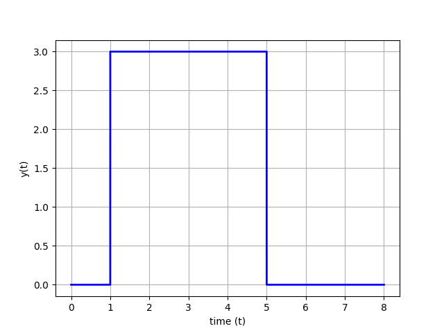
Problem 1a
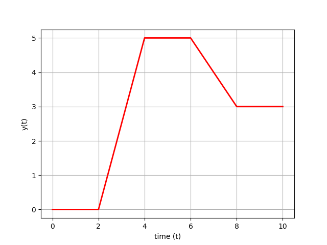
Problem 1b
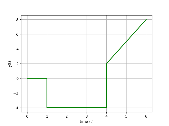
Problem 1c
plt.figure(1)
plt.plot([0,1,1.001,5,5.001,8],[0,0,3,3,0,0],'b-',linewidth=2)
plt.ylabel('y(t)')
plt.xlabel('time (t)')
plt.grid()
plt.savefig('fig1.png')
plt.figure(2)
plt.plot([0,2,4,6,8,10],[0,0,5,5,3,3],'r-',linewidth=2)
plt.ylabel('y(t)')
plt.xlabel('time (t)')
plt.grid()
plt.savefig('fig2.png')
plt.figure(3)
plt.plot([0,1,1.0001,4,4.0001,6],[0,0,-4,-4,2,8],'g-',linewidth=2)
plt.ylabel('y(t)')
plt.xlabel('time (t)')
plt.grid()
plt.savefig('fig3.png')
plt.show()
Problem 2 - Create a Laplace transform expression `F(s)` for the following mathematical functions in the time-domain `f(t)`. See the Laplace Transform table for common transforms.
Problem 2a
$$f(t) = 8 \, t$$
Problem 2b
$$f(t) = 2 \, S\left(t-3\right)$$
`S(t)` is a step function with `S(t\le0)=0` and `S(t\gt0)=1`.
Problem 2c
$$f(t) = 5 \, \frac{dy(t)}{dt}$$
Problem 2d
$$f(t) = 5 \, \int y(t) \, dt$$
Problem 3 - Transform the elements of the following differential equations in time domain into an equivalent differential equation in the Laplace domain. Because the Laplace transform is a linear operator, each element can be transformed separately. Rearrange the equation in the Laplace domain and perform an inverse Laplace transform to solve for an analytic expression of `y(t)`.
Problem 3a
$$\frac{dy(t)}{dt} = -k \, y(t)$$
where k is a constant and with the initial condition `y(0)=5`.
Problem 3b
$$\frac{d^2y(t)}{dt^2} + 2 \, \frac{dy(t)}{dt} + y(t) = 5$$
with initial conditions `y(0)=0`, `\frac{dy(0)}{dt}=0`, and `\frac{d^2y(0)}{dt^2}=0`.
Problem 3c
A first-order linear differential equation is shown as a function of time with constants `\tau` and `K` and variables `y(t)` and `u(t)`. Assume zero initial conditions for the variables.
$$\tau \frac{dy(t)}{dt} = -y(t) + K \, u(t)$$
Derive an analytic solution for `y(t)` with input doublet `u(t)` from Problem 1a.
Create a plot of `y(t)` and `u(t)` with constant values `K=1` and `\tau=2`.
Correction: The video solution is incorrect for problem 2b and 3b. It is `2/s e^{-3s}` for 2b and it is `5/s` (not just 5) on the right side of the equation when performing the Laplace transform of a constant.
Problem 3 Solution Help
The first step is to apply the Laplace transform to each of the terms in the differential equation. Because the Laplace transform is a linear operator, each term can be transformed separately. With a zero initial condition the value of y is zero at the initial time or y(0)=0.
$$\mathcal{L}\left(\tau_p \frac{dy(t)}{dt}\right) = \tau_p \left(s \, Y(s) - y(0)\right) = \tau_p s \, Y(s)$$
$$\mathcal{L}\left(-y(t)\right) = -Y(s)$$
$$\mathcal{L}\left(K \, u(t)\right) = K \, U(s)$$
Putting these terms together gives the first-order differential equation in the Laplace domain.
$$\tau \, s \, Y(s) = -Y(s) + K \, U(s)$$
The differential equation as a function of time (t) is now an algebraic equation in the Laplace domain (s) that can be further manipulated into Transfer Function form. Transfer functions are covered in the next lecture and help built more complex descriptions of dynamic systems.
import numpy as np
K = 1
tau = 2.0
n = 81
t = np.linspace(0,8,n)
s1 = np.zeros(n)
s1[11:] = 1.0
s2 = np.zeros(n)
s2[51:] = 1.0
y = 3*K*(1-np.exp(-(t-1)/tau))*s1 \
-3*K*(1-np.exp(-(t-5)/tau))*s2
plt.figure(1)
plt.plot([0,1,1.001,5,5.001,8],[0,0,3,3,0,0],'b-',linewidth=2)
plt.plot(t,y,'r--')
plt.ylabel('y(t)')
plt.xlabel('time (t)')
plt.legend(['u(t)','y(t)'])
plt.grid()
plt.savefig('fig1.png')
plt.show()
What to Turn In
- Problem 1: Laplace transform expressions F(s) for each graphical time-domain function (1a–1c) using the Laplace Transform table.
- Problem 2: Laplace transform expressions for each mathematical function (2a–2d), showing intermediate steps.
- Problem 3: Transformed Laplace-domain equations and inverse Laplace analytic solutions for each differential equation (3a–3c). Python plot of y(t) and u(t) for Problem 3c using K=1 and `\tau`=2, with a brief explanation of the result.