A tubular column is a structural element that consists of a hollow cylinder made of metal, concrete, or other material. It is commonly used in construction to support beams and other building elements and is also used in bridges and other structures. Tubular columns are generally stronger and more efficient than solid columns as they are able to resist torsion, bending, and shear forces.

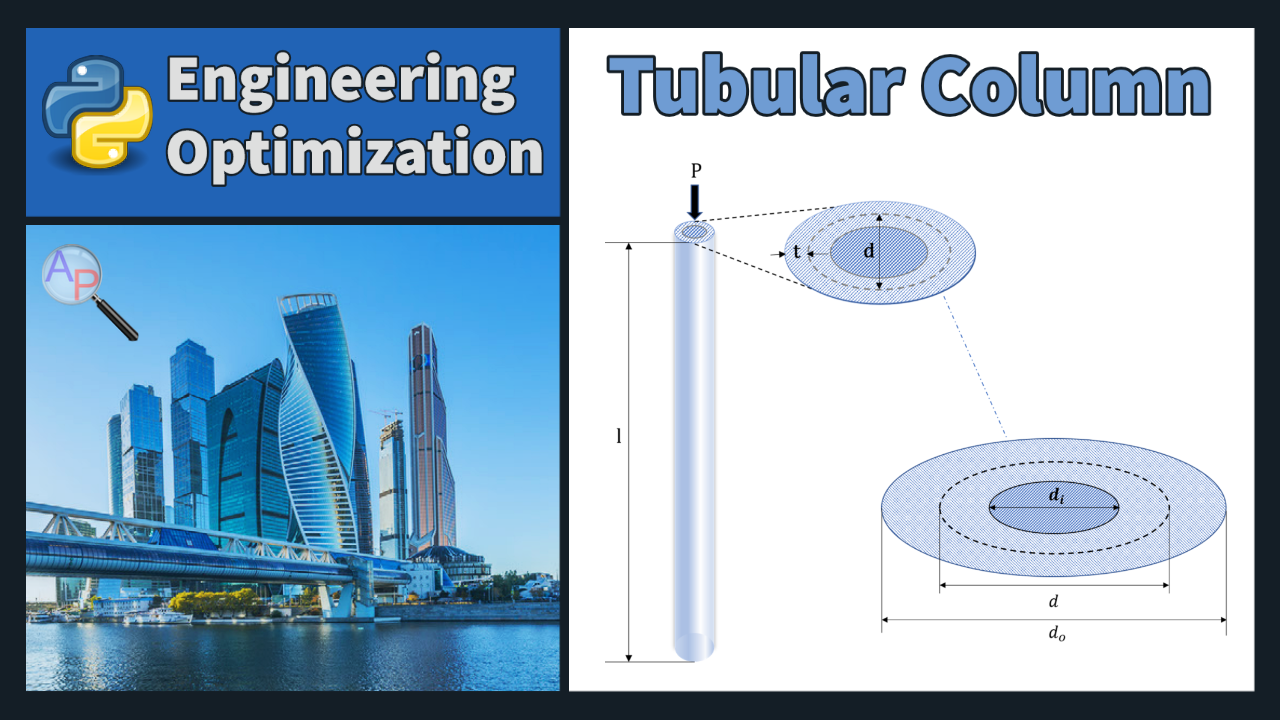
The objective is to optimize the cost of building the column, using variables d, the mean diameter of the column (cm), and t, the thickness of the column (cm).

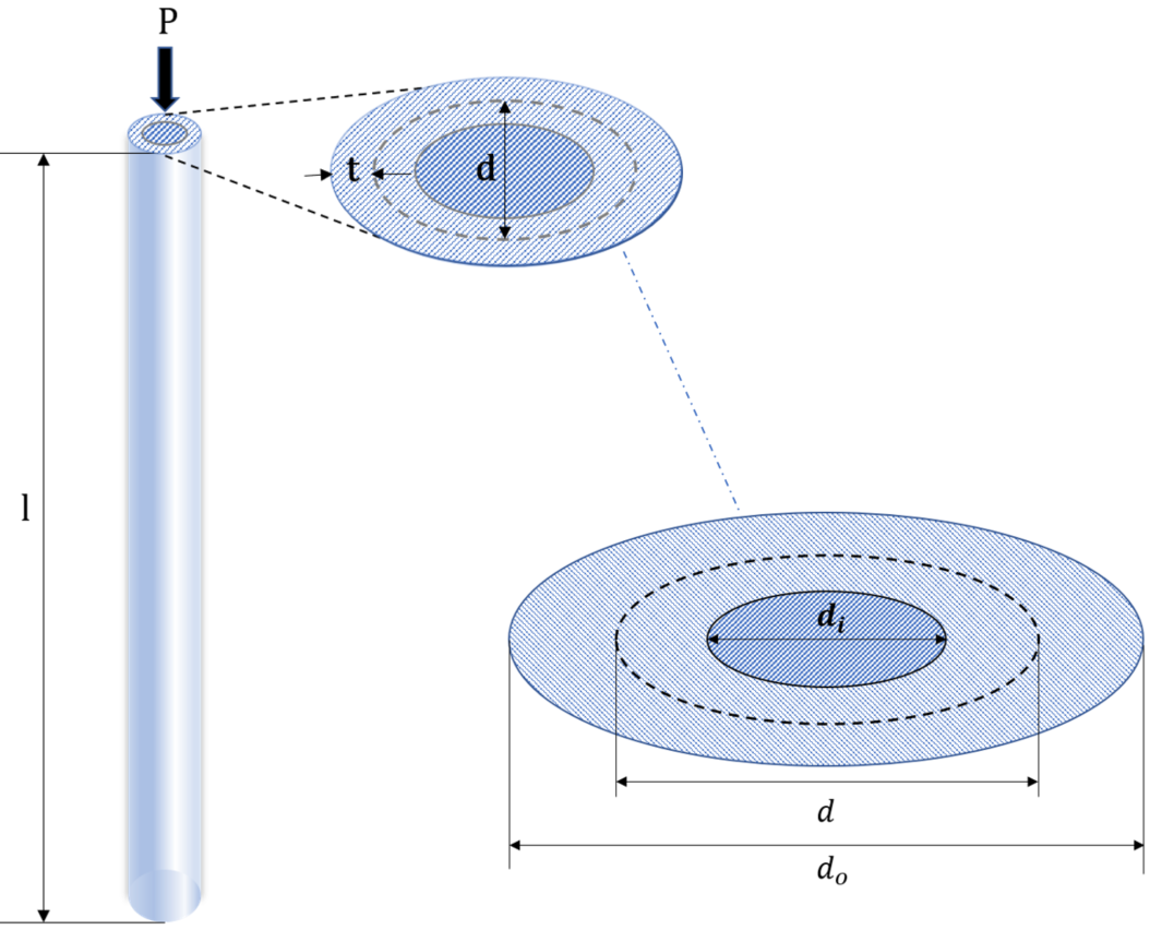
P is the compressive load of 2300 kg_f. The material used to make the column has a module of elasticity (E) of 0.65x10⁶ and a weight density (ρ) of 0.0020 kg_f/cm³. The column has a yield stress (σ_y) of 450 kg_f/cm² and a length (l) of 300 cm.

Due to available materials the diameter must be ≤ 14.0 cm and ≥ 2.0 cm. Similarly, the thickness must be ≤ 0.8 cm and ≥ 0.2 cm. Safety requires that the induced stress is less than the yield stress and that the induced stress is less than the buckling stress. The cost of the column is equal to the expression 5W + 2d with W being the weight in kilograms force (kg_f).

Weight

$$W=\rho l \pi \frac{\left(d_o^2- d_i^2\right)}{4}$$

Outer Diameter

$$d_o=d+t$$

Inner Diameter

$$d_i=d - t$$

Induced stress

$$\frac{P}{\pi\,d \, t}$$

Buckling stress

Buckling stress = Euler buckling load/cross sectional area

$$\frac{\pi^2 E I}{l^2} \frac{1}{\pi \, d \, t}$$

Second moment

Second moment of area of the cross section of the column.

$$I=\frac{\pi}{64} \left(d_0^4- d_i^4\right)$$

Full Tubular Design Assignment (PDF)

Starting Code

Starting code with constants and variables is included below. Fill in the Intermediates, Equations, and Objective Function along with the other necessary commands to solve and analyze this problem.

Solution Report

Turn in a report with the following sections:

1. Title Page with Summary. The Summary should be short (less than 50 words), and give the main optimization results.
2. Procedure: Give a brief description of your model. You are welcome to refer to the assignment which should be in the Appendix. Also include:
   1. A table with the analysis variables, design variables, analysis functions and design functions.
3. Results: Briefly describe the results of optimization (values). Also include:
   1. A table showing the optimum values of variables and functions, indicating binding constraints and/or variables at bounds (highlighted)
   2. A table giving the various starting points which were tried along with the optimal objective values reached from that point.
4. Discussion of Results: Briefly discuss the optimum and design space around the optimum. Do you feel this is a global optimum? Also include and briefly discuss:
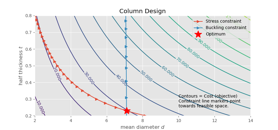
   1. A “zoomed out” contour plot showing the design space (both feasible and infeasible) for diameter and thickness, with the feasible region shaded and optimum marked.
   2. A “zoomed in” contour plot of the design space (mostly feasible space) for diameter and thickness, with the feasible region shaded and optimum marked.
5. Appendix:
   1. Listing of your model with all variables and equations
   2. Solver output with details of the convergence to the optimal values

Any output from the software is to be integrated into the report (either physically or electronically pasted) as given in the sections above. Tables and figures should all have explanatory captions. Do not just staple pages of output to your assignment: all raw output is to have notations made on it. For graphs, you are to shade the feasible region and mark the optimum point. For tables of design values, you are to indicate, with arrows and comments, any variables at bounds, any binding constraints, the objective, etc. (You need to show that you understand the meaning of the output you have included.)

This assignment can be completed in collaboration with others. Additional guidelines on individual, collaborative, and group assignments are provided under the Expectations link.

Solution Help

See GEKKO documentation and additional example problems.

Thanks to Al Duke for providing a solution with a contour plot.

# -*- coding: utf-8 -*-
"""
BYU Intro to Optimization. Column design
https://apmonitor.com/me575/index.php/Main/TubularColumn
Contour plot additions by Al Duke 11/30/2019
"""
from gekko import GEKKO
import matplotlib.pyplot as plt
import numpy as np
from scipy.optimize import fsolve

m = GEKKO()

#%% Constants
pi = m.Const(3.14159,'pi')
P = 2300 # compressive load (kg_f)
o_y = 450 # allowable yield stress (kg_f/cm^2)
E = 0.65e6 # elasticity (kg_f/cm^2)
p = 0.0020 # weight density (kg_f/cm^3)
l = 300 # length of the column (cm)

#%% Variables (the design variables available to the solver)
d = m.Var(value=8.0,lb=2.0,ub=14.0) # mean diameter (cm)
t = m.Var(value=0.3,lb=0.2 ,ub=0.8) # thickness (cm)
cost = m.Var()

#%% Intermediates (computed by solver from design variables and constants)
d_i = m.Intermediate(d - t)
d_o = m.Intermediate(d + t)
W = m.Intermediate(p*l*pi*(d_o**2 - d_i**2)/4) # weight (kgf)
o_i = m.Intermediate(P/(pi*d*t)) # induced stress

# second moment of area of the cross section of the column
I = m.Intermediate((pi/64)*(d_o**4 - d_i**4))

# buckling stress (Euler buckling load/cross-sectional area)
o_b = m.Intermediate((pi**2*E*I/l**2)*(1/(pi*d*t)))

#%% Equations (constraints, etc. Cost could be an intermediate variable)
m.Equations([
o_i - o_y <= 0,
o_i - o_b <= 0,
cost == 5*W + 2*d
])

#%% Objective
m.Minimize(cost)

#%% Solve and print solution
m.options.SOLVER = 1
m.solve()

print('Optimal cost: ' + str(cost[0]))
print('Optimal mean diameter: ' + str(d[0]))
print('Optimal thickness: ' + str(t[0]))

minima = np.array([d[0], t[0]])

#%% Contour plot
# create a cost function as a function of the design variables d and t
f = lambda d, t: 2 * d + 5 * p * l * np.pi * ((d+t)**2 - (d-t)**2)/4

xmin, xmax, xstep = 2, 14, .2 # diameter
ymin, ymax, ystep = .2, .8, .05 # thickness

d, t = np.meshgrid(np.arange(xmin, xmax + xstep, xstep), \
                   np.arange(ymin, ymax + ystep, ystep))
z = f(d, t)

# Determine the compressive stress constraint line.
#stress = P/(pi*d*t) # induced axial stress
t_stress = np.arange(ymin, ymax, .025) # use finer step to get smoother constraint line
d_stress = []
for tt in t_stress:
    dd = P/(np.pi * tt * o_y)
    d_stress.append(dd)

# Determine buckling constraint line. This is tougher because we cannot
#  solve directly for t from d. Used scipy.optimize.fsolve to find roots
d_buck = []
t_buck = []
for d3 in np.arange(6, xmax, .005):
    fb = lambda t : o_y-np.pi**2*E*((d3+t)**4-(d3-t)**4)/(64*l**2*d3*t)
    tr = np.array([0.3])
    roots = fsolve(fb, tr)
    if roots[0] != 0:
        if roots[0] >= .1 and roots[0]<=1.:
            t_buck.append(roots[0])
            d_buck.append(d3)

# Create contour plot
plt.style.use('ggplot') # to make prettier plots
fig, ax = plt.subplots(figsize=(10, 6))

CS = ax.contour(d, t, z, levels=15,)
ax.clabel(CS, inline=1, fontsize=10)
ax.set_xlabel('mean diameter $d$')
ax.set_ylabel('half thickness $t$')

ax.set_xlim((xmin, xmax))
ax.set_ylim((ymin, ymax))

# Add constraint lines and optimal marker
ax.plot(d_stress, t_stress, "->", label="Stress constraint")
ax.plot(d_buck, t_buck, "->", label="Buckling constraint" )

minima_ = minima.reshape(-1, 1)
ax.plot(*minima_, 'r*', markersize=18, label="Optimum")
ax.text(10,.25,"Contours = Cost (objective)\nConstraint line markers point\ntowards feasible space.")
plt.title('Column Design')
plt.legend()
plt.show()

[$[Get Code]]

Generative AI Learning

Use these prompts to test your understanding while completing the exercise. Direct the AI - it may audit and question, but the formulation and runs are yours.

Add to Your Report

Include these items in the solution report described above, in the appropriate sections. You may use Generative AI to help draft and format, but you must supply the correct results, justifications, and assumptions:

1. In Results: your committed pre-run prediction of the active constraint set next to the actual active set from the solver.
2. In Discussion: a unit check of the objective - what units do '5' and '2' carry for cost = 5W + 2d to be consistent, and why does an objective with mixed terms demand this check?
3. In Discussion: re-solve with yield stress 500 instead of 450 kgf/cm^2 and report the change in optimal cost. Interpret the ratio as the yield constraint's shadow price (or explain why the cost did not change).
4. In the Appendix: one question from the quiz prompt you missed and the corrected answer.