Design Optimization

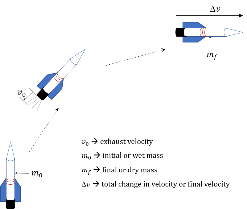
The Tsiolkovsky rocket equation was developed by Russian scientist and pioneer of space exploration, Konstantin Tsiolkovsky. It is a mathematical equation that describes the motion of a rocket in a vacuum and is used to calculate the velocity, acceleration, and thrust of the rocket. The equation is used to determine the optimal design parameters for a rocket and is an important tool for the design of space flight systems.

The Tsiolkovsky rocket [1] has a direct correlation between the change of velocity `(\Delta v)` of a rocket, wet mass `(m_0)`, dry mass `(m_f)`, and exhaust velocity `(v_0)` as shown in:

$$\Delta v = v_0\log{\frac{m_0}{m_f}}$$

This problem optimizes the design of a simple rocket for profit. Potential revenue increases with greater change in velocity, as greater velocities allow the payload to reach higher orbits that have less drag, allowing it to remain in orbit longer. Wet mass, dry mass, and exhaust velocity are design variables, where wet mass is the total initial mass of the rocket, including propellant, and dry mass is the mass of the rocket at full ascent.

The rocket must have a dry mass of at least 20,000 kilograms and the change in velocity should be between 9,400 meters per second and 20,200 meters per second. Varying designs allow for exhaust velocities ranging from 2,500 m/s to 4,500 m/s [2]. An appropriate guess value for the wet mass is 150,650 kilograms.

The overall profit from the rocket is:

$$Profit = R - C_f - C_d - C_e$$

where `C_{f}` is the cost of fuel, given by:

$$C_{f} = 4.154(m_0 - m_f)$$

`C_d` is the cost of the rocket:

$$C_{d} = 154.36 \, m_f$$

`C_{ex}` is the cost in relation to adjusting the exhaust velocity

$$C_{ex} = 75 \, v_0$$

R is revenue and is given by

$$R = 550\Delta v$$

Full Rocket Launch Design Assignment (PDF)

Turn in a report with the following sections:

1. Title Page with Summary. The Summary should be short (less than 50 words), and give the main optimization results.
2. Procedure: Give a brief description of your model. You are welcome to refer to the assignment which should be in the Appendix. Also include:
   1. A table with the analysis variables, design variables, analysis functions and design functions.
3. Results: Briefly describe the results of optimization (values). Also include:
   1. A table showing the optimum values of variables and functions, indicating binding constraints and/or variables at bounds (highlighted)
   2. A table giving the various starting points which were tried along with the optimal objective values reached from that point.
4. Discussion of Results: Briefly discuss the optimum and design space around the optimum. Do you feel this is a global optimum? Also include and briefly discuss:
   1. A “zoomed out” contour plot showing the design space (both feasible and infeasible) for diameter and thickness, with the feasible region shaded and optimum marked.
   2. A “zoomed in” contour plot of the design space (mostly feasible space) for diameter and thickness, with the feasible region shaded and optimum marked.
5. Appendix:
   1. Listing of your model with all variables and equations
   2. Solver output with details of the convergence to the optimal values

Any output from the software is to be integrated into the report (either physically or electronically pasted) as given in the sections above. Tables and figures should all have explanatory captions. Do not just staple pages of output to your assignment: all raw output is to have notations made on it. For graphs, you are to shade the feasible region and mark the optimum point. For tables of design values, you are to indicate, with arrows and comments, any variables at bounds, any binding constraints, the objective, etc. (You need to show that you understand the meaning of the output you have included.)

References

1. Holli Riebeek. Catalog of earth satellite orbits: Feature articles. 2009.
2. Nesrin Sarigul-Klijn, Chris Noel, and Martinus Sarigul-Klijn. Air launching eart-to-orbit vehicles: Delta V gains from launch conditions and vehicle aerodynamics. 01 2004.

Acknowledgement

Thanks to Adam Martin for providing the problem statement and the solution.

This assignment can be completed in collaboration with others. Additional guidelines on individual, collaborative, and group assignments are provided under the Expectations link.

Solution Help

See GEKKO documentation and additional example problems.