Dynamic estimation involves fitting parameters in a dynamic model. In many cases, a linear first order differential equation can approximate the dynamic evolution of many systems. The unknown parameters for this system include the time constant (tau), gain (K), and sometimes dead-time (theta).

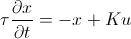
For this exercise, you can assume that the dead-time (theta) is zero and estimate only the time constant (tau) and gain (K). The following data set was generated in class from a voltage input (u) that changed the temperature (x) of a thermister.

• Download Dynamic Data

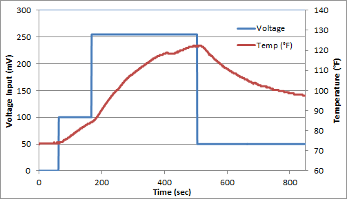
Fit the dynamic data to a first order linear system by estimating tau (time constant) and K (gain). Determine the 95% and 99% confidence intervals for the parameters (see F-test video tutorial).

Excel Solution

The dynamic model can be written in discrete form by specifying that the voltage is constant between sampling intervals. The discrete form of the equation accounts for non-zero initial conditions in temperature (x₀) and voltage (u₀). In this case, the voltage does start at zero, but this is not required.

In this equation, the subscripts denote the sampling intervals that are collected at a time interval of delta time = t_k-t_k-1. The above equation and the data are put into an Excel worksheet. The difference between the measured and predicted values are minimized to obtain the optimal parameters K (gain) and tau (time constant).

• Download Excel Worksheet for Dynamic Parameter Estimation

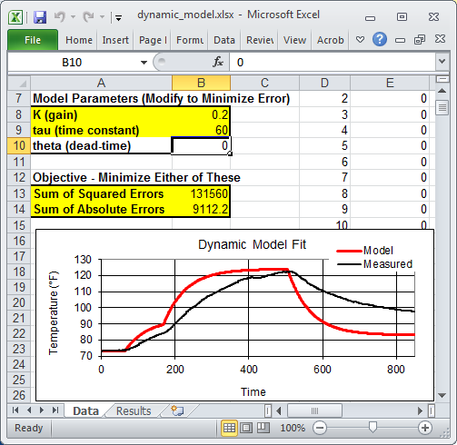
The spreadsheet is currently showing non-optimal values. To obtain the optimal values, use Excel Solver available from the Data toolbar. If the solver option does not appear, it can be added with the Add-In manager.

MATLAB and Python Solutions

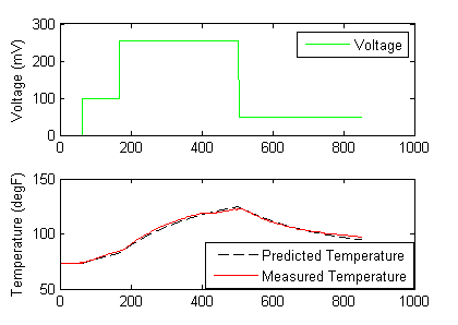
An alternative approach to the sum of squared errors is to minimize an L₁-norm error to find the optimal values of K (gain) and tau (time constant).

• Download MATLAB and Python Solutions for Dynamic Parameter Estimation

The required Python packages are Python, Numpy, Matplotlib, and Scipy. The MATLAB and Python plots produce trends that show the optimal solution with an l₁-norm objective function.

The nonlinear confidence interval is shown by producing a contour plot of the SSE objective function with variations in the two parameters. The optimal solution is shown at the center of the plot and the objective function becomes worse (higher) away from the optimal solution.

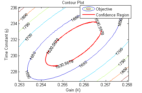
The confidence interval is determined with an F-test that specifies an upper limit to the deviation from the optimal solution

with p=2 (number of parameters), n=851 (number of measurements), theta=[K,tau] (parameters), theta^* as the optimal parameters, SSE as the sum of squared errors, and the F statistic that has 3 arguments (alpha=confidence level, degrees of freedom 1, and degrees of freedom 2). For many problems, this creates a multi-dimensional nonlinear confidence region. In the case of 2 parameters, the nonlinear confidence region is a 2-dimensional space.

The difficulty of the last few assignments has been reduced to allow time for work on the Final Project. Please use the additional time this week to develop the project and start the write-up.

This assignment can be completed in groups of two. Additional guidelines on individual, collaborative, and group assignments are provided under the Expectations link.

Generative AI Learning

Use these prompts to test your understanding after completing the exercise. Direct the AI - it may help with code mechanics, but you must own the estimation setup and the statistical interpretation.

Tip: The estimation-verification loop here is the same one used to calibrate digital twins of batteries, reactors, and buildings: fit parameters, inspect residuals, quantify uncertainty, and only then trust the model for optimization. Fit with both L2 and L1 objectives and compare - if the two disagree noticeably, find the data points responsible.

What to Turn In

Submit a short report (PDF, 1-2 pages) that curates your results into a demonstration of what you learned. You may use Generative AI to help write the report, but you must guide it to the correct fits, statistics, and interpretations. Answer these questions:

1. Report the estimated K and tau with the fit plot (measured vs predicted temperature) and the objective value. State the solver and initial guesses used.
2. Include the confidence-region contour plot for 95% and 99%. Is the region elongated, and what does its shape say about the identifiability of K vs tau?
3. Show the residual plot and judge it: noise or structural mismatch? What model extension would you try if it is structural?
4. Compare L2 and L1 estimates. Do they differ, and which data points explain the difference?
5. From the skeptic prompt: what experiment change did you propose to shrink the confidence region, and why would it work?