Quasi Newton Methods in Optimization
Quasi-Newton methods are a class of numerical optimization algorithms that are used to find minima or maxima of functions. They are a generalization of Newton's method, which uses the Hessian matrix of second derivatives to approximate the local curvature of a function. Quasi-Newton methods use approximate versions of the Hessian matrix that are updated as the algorithm proceeds. This allows the algorithm to more quickly converge to the optimum without needing to compute the full Hessian matrix. The most commonly used quasi-Newton methods are the Broyden–Fletcher–Goldfarb–Shanno (BFGS) and the limited memory BFGS (L-BFGS).
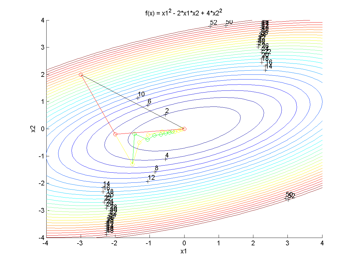
The following exercise demonstrates the use of Quasi-Newton methods, Newton's methods, and a Steepest Descent approach to unconstrained optimization. The following tutorial covers:
- Newton's method (exact 2nd derivatives)
- BFGS-Update method (approximate 2nd derivatives)
- Conjugate gradient method
- Steepest descent method
Chapter 3 covers each of these methods and the theoretical background for each. The following exercise is a practical implementation of each method with simplified example code for instructional purposes. The examples do not perform line searching which will be covered in more detail later.
MATLAB Source Code
 Newton's method
 Steepest descent
 Conjugate gradient
 BFGS update
Python Source Code
 Newton's method
 Steepest descent
 Conjugate gradient
 BFGS update
import numpy as np
import matplotlib.pyplot as plt
# define objective function
def f(x):
x1 = x[0]
x2 = x[1]
obj = x1**2 - 2.0 * x1 * x2 + 4 * x2**2
return obj
# define objective gradient
def dfdx(x):
x1 = x[0]
x2 = x[1]
grad = []
grad.append(2.0 * x1 - 2.0 * x2)
grad.append(-2.0 * x1 + 8.0 * x2)
return grad
# Exact 2nd derivatives (hessian)
H = [[2.0, -2.0],[-2.0, 8.0]]
# Start location
x_start = [-3.0, 2.0]
# Design variables at mesh points
i1 = np.arange(-4.0, 4.0, 0.1)
i2 = np.arange(-4.0, 4.0, 0.1)
x1_mesh, x2_mesh = np.meshgrid(i1, i2)
f_mesh = x1_mesh**2 - 2.0 * x1_mesh * x2_mesh + 4 * x2_mesh**2
# Create a contour plot
plt.figure()
# Specify contour lines
lines = range(2,52,2)
# Plot contours
CS = plt.contour(x1_mesh, x2_mesh, f_mesh,lines)
# Label contours
plt.clabel(CS, inline=1, fontsize=10)
# Add some text to the plot
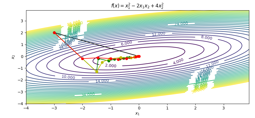
plt.title(r'$f(x)=x_1^2 - 2x_1x_2 + 4x_2^2$')
plt.xlabel(r'$x_1$')
plt.ylabel(r'$x_2$')
##################################################
# Newton's method
##################################################
xn = np.zeros((2,2))
xn[0] = x_start
# Get gradient at start location (df/dx or grad(f))
gn = dfdx(xn[0])
# Compute search direction and magnitude (dx)
# with dx = -inv(H) * grad
delta_xn = np.empty((1,2))
delta_xn = -np.linalg.solve(H,gn)
xn[1] = xn[0]+delta_xn
plt.plot(xn[:,0],xn[:,1],'k-o')
##################################################
# Steepest descent method
##################################################
# Number of iterations
n = 8
# Use this alpha for every line search
alpha = 0.15
# Initialize xs
xs = np.zeros((n+1,2))
xs[0] = x_start
# Get gradient at start location (df/dx or grad(f))
for i in range(n):
gs = dfdx(xs[i])
# Compute search direction and magnitude (dx)
# with dx = - grad but no line searching
xs[i+1] = xs[i] - np.dot(alpha,dfdx(xs[i]))
plt.plot(xs[:,0],xs[:,1],'g-o')
##################################################
# Conjugate gradient method
##################################################
# Number of iterations
n = 8
# Use this alpha for the first line search
alpha = 0.15
neg = [[-1.0,0.0],[0.0,-1.0]]
# Initialize xc
xc = np.zeros((n+1,2))
xc[0] = x_start
# Initialize delta_gc
delta_cg = np.zeros((n+1,2))
# Initialize gc
gc = np.zeros((n+1,2))
# Get gradient at start location (df/dx or grad(f))
for i in range(n):
gc[i] = dfdx(xc[i])
# Compute search direction and magnitude (dx)
# with dx = - grad but no line searching
if i==0:
beta = 0
delta_cg[i] = - np.dot(alpha,dfdx(xc[i]))
else:
beta = np.dot(gc[i],gc[i]) / np.dot(gc[i-1],gc[i-1])
delta_cg[i] = alpha * np.dot(neg,dfdx(xc[i])) + beta * delta_cg[i-1]
xc[i+1] = xc[i] + delta_cg[i]
plt.plot(xc[:,0],xc[:,1],'y-o')
##################################################
# Quasi-Newton method
##################################################
# Number of iterations
n = 8
# Use this alpha for every line search
alpha = np.linspace(0.1,1.0,n)
# Initialize delta_xq and gamma
delta_xq = np.zeros((2,1))
gamma = np.zeros((2,1))
part1 = np.zeros((2,2))
part2 = np.zeros((2,2))
part3 = np.zeros((2,2))
part4 = np.zeros((2,2))
part5 = np.zeros((2,2))
part6 = np.zeros((2,1))
part7 = np.zeros((1,1))
part8 = np.zeros((2,2))
part9 = np.zeros((2,2))
# Initialize xq
xq = np.zeros((n+1,2))
xq[0] = x_start
# Initialize gradient storage
g = np.zeros((n+1,2))
g[0] = dfdx(xq[0])
# Initialize hessian storage
h = np.zeros((n+1,2,2))
h[0] = [[1, 0.0],[0.0, 1]]
for i in range(n):
# Compute search direction and magnitude (dx)
# with dx = -alpha * inv(h) * grad
delta_xq = -np.dot(alpha[i],np.linalg.solve(h[i],g[i]))
xq[i+1] = xq[i] + delta_xq
# Get gradient update for next step
g[i+1] = dfdx(xq[i+1])
# Get hessian update for next step
gamma = g[i+1]-g[i]
part1 = np.outer(gamma,gamma)
part2 = np.outer(gamma,delta_xq)
part3 = np.dot(np.linalg.pinv(part2),part1)
part4 = np.outer(delta_xq,delta_xq)
part5 = np.dot(h[i],part4)
part6 = np.dot(part5,h[i])
part7 = np.dot(delta_xq,h[i])
part8 = np.dot(part7,delta_xq)
part9 = np.dot(part6,1/part8)
h[i+1] = h[i] + part3 - part9
plt.plot(xq[:,0],xq[:,1],'r-o')
plt.savefig('contour.png')
plt.show()
More Advanced Solvers
The above implementations are very simple with 7-30 lines of code each. More advanced methods are implemented with Nonlinear Programming (NLP) and Mixed Integer Nonlinear Programming Solvers (MINLP) solvers such as APOPT (MINLP solver), BPOPT (NLP solver), and IPOPT (NLP solver). The following Python Gekko code demonstrates the performance with these three solvers by changing m.options.SOLVER to 1=APOPT, 2=BPOPT, 3=IPOPT.
m = GEKKO()
x1 = m.Var(-3)
x2 = m.Var(2)
m.Minimize(x1**2-2*x1*x2+4*x2**2)
m.options.SOLVER = 2 # 1=APOPT, 2=BPOPT, 3=IPOPT
m.solve()
print(x1.value[0],x2.value[0])
The simple objective only requires an unconstrained Quadratic Programming (QP) solver with the objective function.
$$\min_{x_1,x_2} \left(x_1^2-2 x_1 x_2 + 4 x_2^2\right)$$
The NLP and MINLP solvers can also solve the problem. APOPT converges in 4 iterations using 1st derivatives, BPOPT converges in 3 iterations with 1st and 2nd derivatives, and IPOPT converges in 2 iterations with 1st and 2nd derivatives.
 This assignment can be completed in groups of two. Additional guidelines on individual, collaborative, and group assignments are provided under the Expectations link.