Discrete Optimization in Engineering Design
Discrete decision variables are those that have only certain levels or quantities that are acceptable at an optimal solution. Examples of discrete variables are binary (e.g. off/on or 0/1), integer (e.g. 4,5,6,7), or general discrete values that are not integer (e.g. 1/4 cm, 1/2 cm, 1 cm).
One often encounters problems in which design variables must be selected from among a set of discrete values. Examples of discrete variables include catalog or standard sizes (I beams, motors, springs, fasteners, pipes, etc.), materials, and variables which are naturally integers such as people, gear teeth, number of shells in a heat exchanger and number of distillation trays in a distillation column. Many engineering problems are discrete in nature.
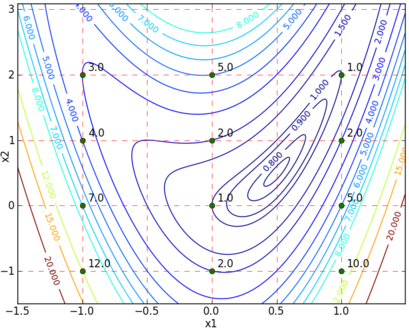
At first glance it might seem solving a discrete variable problem would be easier than a continuous problem. After all, for a variable within a given range, a set of discrete values within the range is finite whereas the number of continuous values is infinite. When searching for an optimum, it seems it would be easier to search from a finite set rather than from an infinite set.
This is not the case, however. Solving discrete problems is harder than continuous problems. This is because of the combinatorial explosion that occurs in all but the smallest problems. For example if we have two variables which can each take 10 values, we have 10*10 = 100 possibilities. If we have 10 variables that can each take 10 values, we have 10^10 possibilities. Even with the fastest computer, it would take a long time to evaluate all of these.
The integer problem can be solved with Python GEKKO. The option integer=True is used to switch the variable from continuous to integer form. The APOPT solver is required to solve problem with integer variables but other solvers such as IPOPT can provide a relaxed solution where the integer conditions are not enforced.
m = GEKKO() # create GEKKO model
# create integer variables
x1 = m.Var(integer=True,lb=-1,ub=1)
x2 = m.Var(integer=True,lb=-1,ub=2)
m.Minimize(4*x1**2-4*x2*x1**2+x2**2+x1**2-x1+1)
m.options.SOLVER = 1 # APOPT solver
m.solve()
print('x1: ' + str(x1.value[0]))
print('x2: ' + str(x2.value[0]))
Discussion Questions
Bring answers to class or work them with an AI tutor - ask it to grade your answer and argue the other side before it explains.
- "Solve the continuous problem, then round to the nearest catalog size." Construct or recall a two-variable example where the rounded design is infeasible AND another where it is feasible but clearly suboptimal. Why does the danger grow with more active constraints?
- In branch and bound, the continuous relaxation at a node gives a bound. For a minimization: is the relaxation's optimum a lower or an upper bound, why can a node be discarded when its bound is worse than the best integer solution found so far, and what would go wrong if the relaxation were solved only approximately?
- A problem has 30 variables, each with 8 catalog values. How many combinations exist, and at one microsecond per evaluation, how long would exhaustive search take? What do these numbers say about why bounding - not raw speed - is the enabling idea?
- Topology optimization for additive manufacturing decides material-or-void in each of millions of cells - the ultimate discrete problem. Modern methods relax it to continuous densities, optimize with gradients, then push densities to 0/1. Connect this strategy to the relaxation idea in branch and bound: what is gained and what optimality guarantee is given up?
