Oxygen Supply Design Optimization
A Basic Oxygen Furnace (BOF) used in steelmaking where a stream of oxygen is blown into a bath of molten iron and scrap steel. This accelerates the oxidation process and removes impurities such as carbon, silicon, manganese, and phosphorus from the steel. The end result is a higher quality steel product.
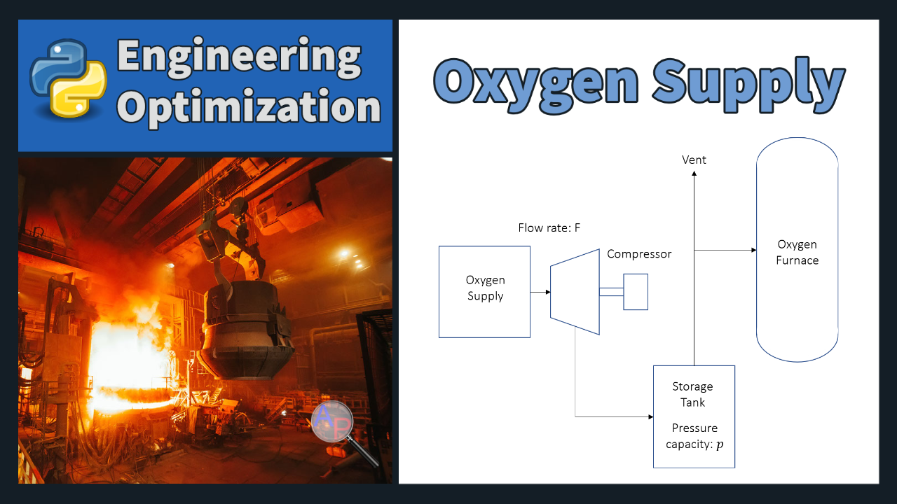
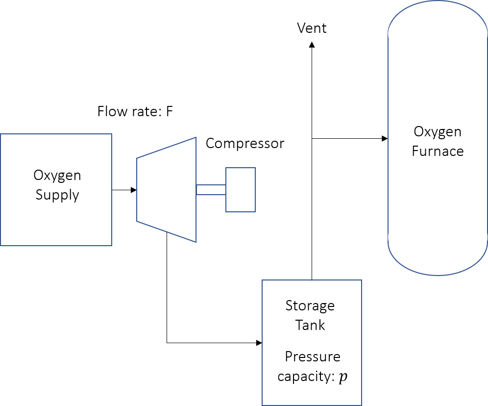
The operation of a BOF is based on cycles. Each cycle consists of a low oxygen demand interval in which raw materials are introduced to the furnace, and a high oxygen demand interval in which the raw material is processed. The low demand interval is 0.4 hours, and the high demand interval (`t_1`) is 0.6 hours, giving a total cycle time (`t_2`) of 1 hour. Due to equipment limitations, the oxygen production rate (`F`) is held constant throughout the cycle. Any excess oxygen produced during the low demand period is compressed and stored, to be withdrawn as needed during the high demand period. The objective of this problem is to design an oxygen-supply and storage system that meets the oxygen demand of the furnace over the entire cycle while minimizing cost. The following figure shows the BOF system.
The two design variables for this system are the maximum storage tank pressure (`p` in psia) and the oxygen production rate (`F` in tons/hour). The given constants are the low oxygen demand rate (`D_0`) at 2.4 tons/hour, the high oxygen demand rate (`D_1`) at 37 tons/hour, the gas constant (`R`) at 670.6 `ft^{3}` psia/(HP-hr), temperature (`T`) at 530 degrees Rankine, the compressibility factor 0.98 (`z`), unit conversion factor (`k_1`) at 14005.8, compressor efficiency (`k_2`) at 0.75, and the oxygen delivery pressure (`p_0`) at 200 psia.
These values are used to calculate the compressor design capacity (`H`) and the storage tank design capacity (`V`). These intermediate values are then used to calculate the total cost of the system.
Annual Cost Function
The annual cost (`AC`) of the BOF system is found using the following equation. The parameter `d` is an annual cost factor for the compressor and storage tank and `N` is the number of cycles in one year of operation.
$$AC = C_1 + (C_2 + C_3)\,d + N\,C_4$$
There are four cost elements. `C_1` is the oxygen plant annual cost `C_1 = a_1 + a_2F`, `C_2` is the capital cost of the storage vessel `C_2 = s_1 s_2 V^{s_3}`, `C_3` is the capital cost of the compressor `C_3 = 0.2 b_1 b_2 H^{b_3}`, and `C_4` is the compressor power cost `C_4 = 0.001 b_4 t_1 H`. In these equations `a_1`, `a_2`, `s_1`, `s_2`, `s_3`, `b_1`, `b_2`, `b_3`, `b_4` are cost parameters.
Table 1: Cost parameters for the oxygen supply and storage system
| Parameter | Value | Units |
| `a_1` | 60.9 | dollars/hour |
| `a_2` | 5.83 | dollars/hour |
| `b_1` | 2.5e-5 | dollars/hour |
| `b_2` | 680 | `HP^{-c_3}` |
| `b_3` | 0.85 | dimensionless |
| `b_4` | 6.0e-3 | dollars/(HP-HR) |
| `s_1` | 3.0e-5 | dollars/hour |
| `s_2` | 660 | `(ft^3)^{-b_3}` |
| `s_3` | 0.9 | dimensionless |
| `d` | 5 | dimensionless |
| `N` | 8000 | dimensionless |
Constraints
The maximum amount of oxygen stored (`I_{max}`) in the tank during the cycle is calculated as:
$$I_{max} = (D_1 - F)\,(t_2 - t_1)$$
The compressor design capacity is given by:
$$H = \frac{I_{max}}{t_1} \frac{RT}{k_1k_2} \ln{(\frac{p}{p_0})}$$
The maximimum design tank pressure has a lower bound as given by the following constraint:
$$p >= p_0 + 1$$
To meet the required oxygen demand the production rate must meet the following constraint:
$$F >= \frac{D_0 \, t_1 + D_1 \, (t_2 - t_1)}{t_2}$$
Full Problem Statement
Full Oxygen Supply Design Assignment (PDF)
Assignment
Turn in a report with the following sections:
- Title Page with Summary. The Summary should be short (less than 50 words), and give the main optimization results.
- Procedure: Give a brief description of your model. You are welcome to refer to the assignment which should be in the Appendix. Also include:
- A table with the analysis variables, design variables, analysis functions and design functions.
- Results: Briefly describe the results of optimization (values). Also include:
- A table showing the optimum values of variables and functions, indicating binding constraints and/or variables at bounds (highlighted)
- A table giving the various starting points which were tried along with the optimal objective values reached from that point.
- Discussion of Results: Briefly discuss the optimum and design space around the optimum. Do you feel this is a global optimum? Also include and briefly discuss:
- A “zoomed out” contour plot showing the design space (both feasible and infeasible) for diameter and thickness, with the feasible region shaded and optimum marked.
- A “zoomed in” contour plot of the design space (mostly feasible space) for diameter and thickness, with the feasible region shaded and optimum marked.
- Appendix:
- Listing of your model with all variables and equations
- Solver output with details of the convergence to the optimal values
Any output from the software is to be integrated into the report (either physically or electronically pasted) as given in the sections above. Tables and figures should all have explanatory captions. Do not just staple pages of output to your assignment: all raw output is to have notations made on it. For graphs, you are to shade the feasible region and mark the optimum point. For tables of design values, you are to indicate, with arrows and comments, any variables at bounds, any binding constraints, the objective, etc. (You need to show that you understand the meaning of the output you have included.)
References
- A Ravindran, Gintaras Victor Reklaitis, and Kenneth Martin Ragsdell. Engineering optimization: methods and applications. John Wiley & Sons, 2006.
- Frank C. Jen, C. Carl Pegels, and Terrence M. Dupuis. Optimal capacities of production facilities. Management Science, 14(10):B573–B580, 1968.
Acknowledgement
Thanks to Adam Martin for providing the problem statement and the solution.
 This assignment can be completed in collaboration with others. Additional guidelines on individual, collaborative, and group assignments are provided under the Expectations link.
Solution Help

See GEKKO documentation and additional example problems.
m = GEKKO()
#%% Model Oxygen Supply
#Constants
R = 670.6 #gas law (cubic feet-psia/(HP - HR))
T = 530 #Temperature (degrees Rankine)
z = 0.98 #Compressibility factor ()
M = 15.999 #Molecular weight (u)
k_1 = 14005.8 #unit conversion factor
#cycle parameters
N = 8000 #Number of cycles per year
D_0 = 2.4 #Low demand rate of O_2 (tons/hr)
D_1 = 37 #High demand rate of O_2 (tons/hr)
t_1 = 0.6 #time interval of high demand rate
t_2 = 1 #time interval of one cycle of low and high demand rate
#cost parameters
a_1 = 60.9
a_2 = 5.83
b_1 = 2.5e-5
b_2 = 680
b_3 = 0.85
b_4 = 6.0e-3 #cost of power
s_1 = 3.0e-5
s_2 = 374
s_3 = 0.9
d = 5 #annual cost factor
#physical parameters
p_0 = 200 #O_2 delivery pressure
k_2 = 0.75 #Compressor efficiency
#%% Variables
#Independent variables
F = m.Var() #Production rate(tons/hr)
p = m.Var() #Tank pressure (psia)
annual_cost = m.Var() #Objective.
#%% Intermediates
I_max = m.Intermediate((D_1 - F)*(t_2 - t_1))
V = m.Intermediate((I_max/M)*(R*T/p)*z)
H = m.Intermediate((I_max/t_1)*(R*T/(k_1*k_2))*m.log(p/p_0))
#Oxygen plant annual cost
C_1 = m.Intermediate(a_1 + a_2*F)
#Capital cost of storage vessels
C_2 = m.Intermediate(s_1*s_2*V**s_3)
#Capital cost of compressors
C_3 = m.Intermediate(0.2*b_1*b_2*H**b_3)
#Compressor power cost
C_4 = m.Intermediate(0.001*b_4*t_1*H)
#%% Equations
m.Equations([
annual_cost == C_1 + d*(C_2 + C_3) + N*C_4,
F >= (D_0*t_1 + D_1*(t_2 - t_1))/t_2,
p >= p_0 + 1
])
#%% Objective
m.Minimize(annual_cost)
#%% Solve
m.solve()
print("Optimal annual cost:" , str(annual_cost[0]))
print("Optimal production rate:" , str(F[0]))
print("Optimal maximum tank pressure:" , str(p[0]))
