Heat Integration Optimization
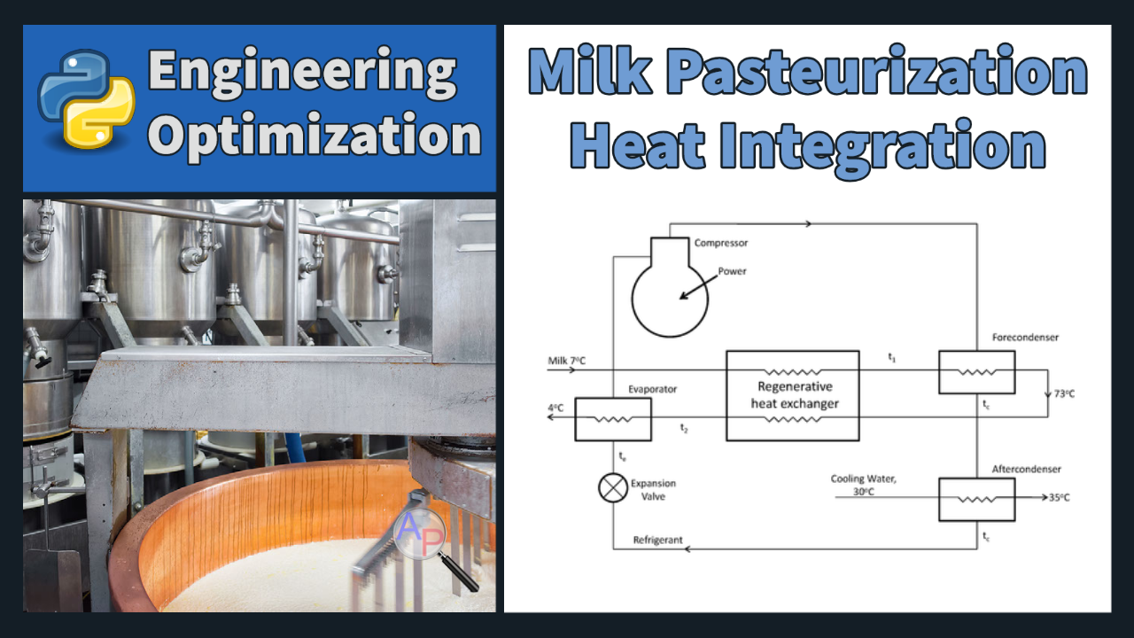
A heat pump is a type of heating and cooling system that uses an external heat source or sink to provide cooling in summer and heating in winter. It can also be used to provide heat for industrial processes such as milk pasteurization. The system works by transferring heat from the source to the milk. The heat exchanger acts as a buffer, to heat the incoming milk and cool the outgoing milk. This type of heat integration is highly efficient and helps to reduce energy costs.
In the pasteurization of milk, the temperature is raised to 73°C, held for 20 sec., and then cooled. The milk arrives at a temperature of 7°C and is delivered from the pasteurizing process for packaging at a temperature of 4°C.
We will consider using a heat pump with a regenerative heat exchanger to do this. One possible cycle is shown in the figure below. The incoming milk is preheated in a regenerative heat exchanger and then heated further in the fore-condenser of the heat pump. As it exits the fore-condenser, the temperature of the milk is 73°C. Thereafter the milk is cooled as it flows through the other side of the regenerative heat exchanger and then through the evaporator of the heat pump.
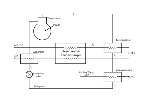
Find the optimal heat pump and regenerative exchanger that minimizes the total present worth of costs (capital cost and operating cost). Specifically, determine the areas of the heat exchangers (evaporator, condensers, and regenerative exchanger), size of the compressor, and temperatures t1, t2, te and tc that result in the minimum total cost. Run the problem with no constraints on temperatures of approach (Case 1); then rerun with constraints that all temperatures of approach (evaporator, condensers, regenerative heat exchanger) are at least 10 °C (Case 2).
This problem is based on a problem from W. Stoecker, Design of Thermal Systems, 3rd ed.
 This assignment can be completed in groups of two. Additional guidelines on individual, collaborative, and group assignments are provided under the Expectations link.
Solution Help

See GEKKO documentation and additional example problems.
# Initialize Gekko model
m = GEKKO()
# Optimal heat pump and regenerative exchanger that minimizes the total present
# worth of costs (capital cost and operating cost). Specifically, determine the
# areas of the heat exchangers (evaporator, condensers, and regenerative
# exchanger), size of the compressor, and temperatures t1, t2, te and tc
# that result in the minimum total cost
# Parameters
U = 0.6
Ureg = 0.5
mdotm = 4
cpm = 3.75
cpw = 1.00
intrate = 0.09
nper = 6
# Inlet temperature (degC)
ti = 7
# Outlet temperature (degC)
to = 4
# Pasteurization Temperature (degC), target temperature
tp = 73
# Variables
# compressor work (kW)
W = m.Var()
# heat exchanger areas (m^2)
Ae = m.Var(value = 10, lb = 1.0, ub = 1000)
Areg = m.Var(value = 10, lb = 1.0, ub = 1000)
Afc = m.Var(value = 10, lb = 1.0, ub = 1000)
Aac = m.Var(value = 10, lb = 1.0, ub = 1000)
t1 = m.Var(value = ti) # Temperature 1 (degC)
t2 = m.Var(value = ti) # Temperature 2 (degC)
te = m.Var(value = ti) # Evaporator Temperature (degC)
tc = m.Var(value = ti) # Condenser Temperature (degC)
Ctot = m.Var(value = 100000) # Total Cost
# evaporator
Qe = m.Var(value = 1)
dapp1e = m.Var(value = 1)
dapp2e = m.Var(value = 1)
# regenerative heat exchanger
Qreg = m.Var(value = 1)
dapp1reg = m.Var(value = 1)
dapp2reg = m.Var(value = 1)
# fore condenser
Qfc = m.Var(value = 1)
dapp1fc = m.Var(value = 1)
dapp2fc = m.Var(value = 1)
# after condenser
Qac = m.Var(value = 1)
dapp1ac = m.Var(value = 1)
dapp2ac = m.Var(value = 1)
# temps of approach
dappe = m.Var(lb = 0.1) # >= 10
dappc = m.Var(lb = 0.1) # >= 10
dappreg1 = m.Var(lb = 0.1) # >= 10
dappreg2 = m.Var(lb = 0.1) # >= 10
# ratios
ratio_e = m.Var(value = .05, lb = 0.001, ub = 0.999)
ratio_reg = m.Var(value = .05, lb = 0.000, ub = 1.0)
ratio_fc = m.Var(value = .05, lb = 0.001, ub = 0.999)
ratio_ac = m.Var(value = .05, lb = 0.001, ub = 0.999)
# Log-mean temperature differences
delte = m.Var(value = 1)
deltreg = m.Var(value = 1)
deltfc = m.Var(value = 1)
deltac = m.Var(value = 1)
# Coefficient Of Performance
COP = m.Var(value = 1)
# Intermediates
# Cost elec year at 4 hours per day
Celyear= m.Intermediate(W * 4.0 * 365.0 * 0.07)
# Cost total over time
# Multiplier is about 4.5 (instead of 6.0) because of the
# interest rate on unspent capital
mult = m.Intermediate((((1.0+intrate)**nper)-1.0) / (intrate*(1.0+intrate)**nper))
Celtot = m.Intermediate(Celyear * mult)
# Cost equipment
Cequip = m.Intermediate(Ae*200.0 + Afc*200.0 + Aac*200.0 + Areg*200 + W*240.0)
#temperatures in Kelvin
TeK = m.Intermediate(te + 273)
TcK = m.Intermediate(tc + 273)
# Equations
m.Equations([
# Total cost
Ctot == Celtot + Cequip,
# overall energy balance on regen heat exchanger
# mdotm and cpm cancel from each term
t1 + t2 == tp + ti,
# log-mean temperature difference
# lmtd(thi,tco,tho,tci)
# evaporator
Qe == mdotm * cpm *(t2 - to),
dapp1e == to - te,
dapp2e == t2 - te,
# regenerative heat exchanger
Qreg == mdotm * cpm * (tp-t2),
dapp1reg == t2 - ti,
dapp2reg == tp - t1,
# fore condenser
Qfc == mdotm * cpm * (tp - t1),
dapp1fc == tc - tp,
dapp2fc == tc - t1,
# after condenser
Qac == W + mdotm * cpm * (ti - to),
dapp1ac == tc - 35.0,
dapp2ac == tc - 30.0,
# approach temperatures
dappe == to - te, # Temp app evap
dappc == tc - tp, # Temp app fore cond
dappreg1 == t2 - ti, # Temp app reg1
dappreg2 == tp - t1, # Temp app reg2
# ratios
ratio_e * dapp2e == dapp1e,
ratio_reg * dapp2reg == dapp1reg,
ratio_fc * dapp2fc == dapp1fc,
ratio_ac * dapp2ac == dapp1ac,
# Log-mean Temperature Difference
delte * m.log(ratio_e) == (dapp1e - dapp2e),
#deltreg * m.log(ratio_reg) = (dapp1reg - dapp2reg)
deltfc * m.log(ratio_fc) == (dapp1fc - dapp2fc),
deltac * m.log(ratio_ac) == (dapp1ac - dapp2ac),
# Average temperature difference
#delte = (dapp1e + dapp2e) / 2
deltreg == (dapp1reg + dapp2reg) / 2,
#deltfc = (dapp1fc + dapp2fc) / 2
#deltac = (dapp1ac + dapp2ac) / 2
# coefficient of performance
# 75% of Carnot Efficiency
COP * (TcK-TeK) == 0.75 * TeK,
# Work to compressor
W * COP == Qe,
# heat transferred for each exchanger
Ae * U * delte == Qe,
Areg * Ureg * deltreg == Qreg,
Afc * U * deltfc == Qfc,
Aac * U * deltac == Qac
])
# objective function
m.Minimize(Ctot)
# minimize ctot
m.options.SOLVER = 1
m.options.IMODE = 3
m.solve()
print('Minimum cost: ' + str(Ctot[0]))
Generative AI Learning
Use these prompts to test your understanding after completing the exercise. Direct the AI - it may probe your model, but the energy balances and the optimization are yours.
Tip: Before optimizing, hand-check your energy balances at a fixed design: pick t1 = 40 C and verify every duty (kW) and area (m^2) with a calculator. An optimizer pointed at a wrong model finds the wrong optimum with great precision.
What to Turn In
Submit a short report (PDF, 1-2 pages) that curates your results into a demonstration of what you learned. You may use Generative AI to help write the report, but you must guide it to the correct energy balances, justifications, and assumptions. Answer these questions:
- Present the optimal design for both cases (areas, compressor size, temperatures t1, t2, te, tc) and the total present worth of each. Where does the extra cost of Case 2 come from?
- Show your hand verification of the energy balance at one fixed design point. Did it catch anything wrong in your model?
- Which constraints are active in Case 2, and what is the economic meaning of the multiplier on one active approach-temperature constraint (dollars per degree of approach)?
- How does the optimum shift if electricity rises from $0.07 to $0.10 per kWh? Report re-optimized results and explain the direction of every change.
- From the quiz prompt: one question you missed and the corrected answer.
