Limestone Slurry Pipeline Optimization
A slurry pipeline transports a mixture of materials suspended in a liquid or gas. These materials are usually particles of solid matter, such as sand, clay, and other minerals, suspended in a liquid base, such as water or oil. Slurry pipelines are used in many industries, including mining, oil and gas, and agriculture.
The optimization of a slurry pipeline depends on the type of slurry and the application. In general, the goal is to minimize the total cost of the pipeline, which includes capital and operating costs. Optimization may involve adjusting the diameter of the pipeline, the type and number of pumps, the use of valves and other controlling devices, and the installation of strainers and other equipment to filter out solids. Other considerations include the environmental impact of the pipeline, safety, and the ability to handle the slurry without damage to the equipment. In some cases, the optimization process may also include the use of additives to improve the flow characteristics of the slurry.
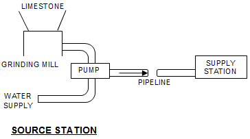
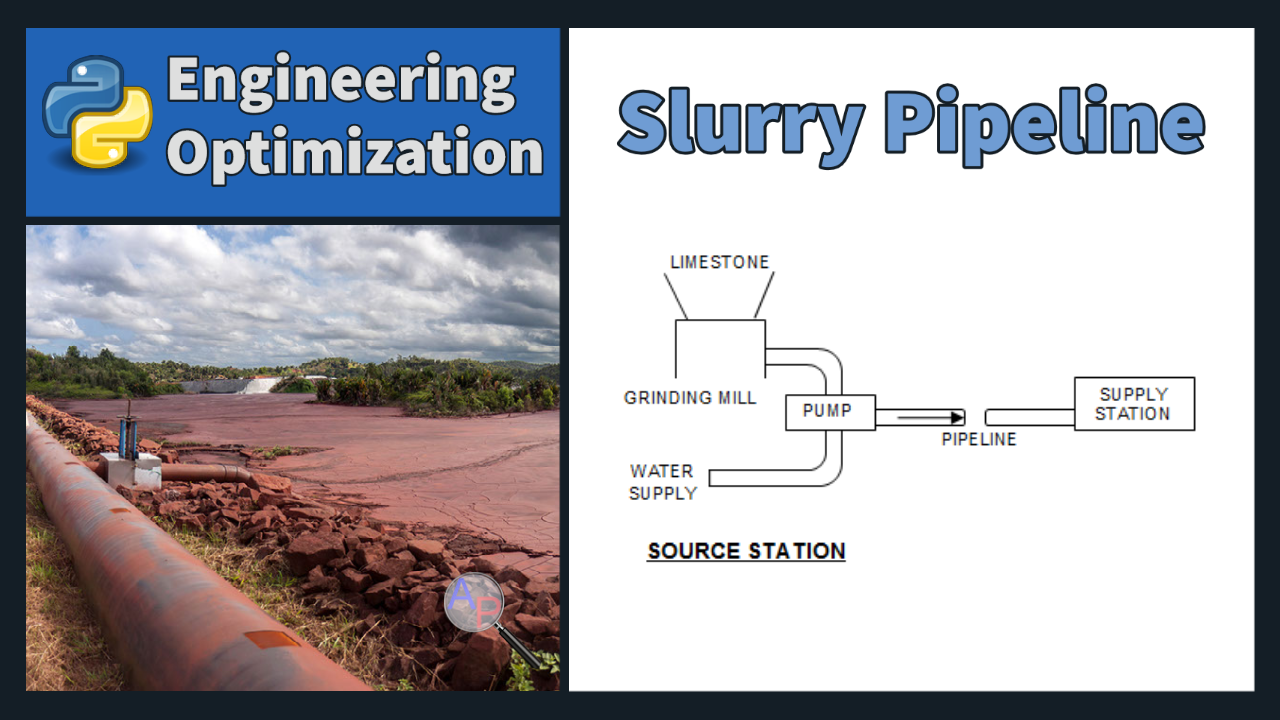
Design a pipeline for transporting crushed limestone from a quarry to a terminal located some distance away, using water as a transporting medium.
Part of the optimization model requires an empirical model of Cd vs. CdRp2 to correctly size the slurry pump. There are several methods for obtaining a regression model of this relationship including a cubic spline or machine learning regression methods. Gekko (see documentation) imports TensorFlow, Scikit-Learn, and Gaussian Process models.
| CdRp2 | Cd |
|---|---|
| 2.4 | 240 |
| 4.8 | 120 |
| 7.2 | 80 |
| 12.4 | 49.5 |
| 17.9 | 36.5 |
| 26.5 | 26.5 |
| 58.4 | 14.6 |
| 93.7 | 10.4 |
| 173 | 6.9 |
| 260 | 5.3 |
| 410 | 4.1 |
| 1020 | 2.55 |
| 1800 | 2 |
| 3750 | 1.5 |
| 6230 | 1.27 |
| 10,700 | 1.07 |
| 30,800 | 0.77 |
| 58,500 | 0.65 |
| 138,000 | 0.55 |
| 245,000 | 0.5 |
| 460,000 | 0.46 |
| 1,680,000 | 0.42 |
| 3,600,000 | 0.4 |
| 9,600,000 | 0.385 |
The limestone is crushed at the quarry, mixed with water to form a slurry, and pumped through the pipe. We would like to minimize the operating cost, which is primarily determined by the grinding power and the pumping power.
This problem is taken from James Siddall, Optimal Engineering Design, Dekker.
 This assignment can be completed in groups of two. Additional guidelines on individual, collaborative, and group assignments are provided under the Expectations link.
Solution Help

See GEKKO documentation and additional example problems.
from gekko import GEKKO
m = GEKKO()
# Slurry Pipeline
# Constants
L = 15*5280 # Length of pipeline (ft)
W = 12.67 # Massflow of limestone (lbm/sec)
a = 0.01 # Average lump-size before grinding (ft)
pi = 3.1415927
rho_w = 62.428 # Density of water (lbm/ft^3)
mu = 7.392e-4 # Viscosity of water (lbm/ft/sec)
g = 32.174 # Gravitational constant (ft/sec^2)
# Conversion between lbm and lbf (lbm ft / lbf / s^2)
gc = 32.174049
# Density of limestone (lbm/ft^3)
gamma_L = 168.5
# Variables
# Average flow velocity (ft/sec)
V = m.Var(value=10, lb=1, ub=20, name='V')
# Volumetric concentration of slurry
# (Vol limestone/Vol Total)
c = m.Var(value=0.2, lb=0.01, ub=0.4, name='c')
# Internal pipe diameter (ft)
Dpipe = m.Var(value=0.4, lb=0.01, ub=0.5, name='Dpipe')
# Average particle size after grinding (ft)
d = m.Var(value=0.008, lb=0.0008, name='d')
Pt = m.Var(value=1, name='Pt')
# Intermediates
# Reynolds number
Rw = m.Intermediate(rho_w*V*Dpipe/mu)
# Friction factor
ffp = True
if ffp:
y = m.Intermediate(m.log(Rw))
fw = m.Intermediate(-1.5919e-4*y**3+5.5535e-3*y**2\
-6.8029e-2*y+0.31078)
else:
fw1 = 0.3164/(Rw**0.25)
fw2 = 0.0032+0.221*Rw**-0.237
fw = m.if3(Rw-1e5,fw1,fw2)
# Dimensionless numbers to obtain drag coefficient
cspline = True
CdRp2 = m.Intermediate(4*g*rho_w*d**3*\
(gamma_L-rho_w)/(3*mu**2))
if cspline:
import pandas as pd
course = 'http://apmonitor.com/me575/'
url = 'index.php/Main/LimestoneSlurry'
data = pd.read_html(course+url)[0] # read data
lnCdRp2,lnCd,Cd = m.Array(m.Var,3,value=2)
m.Equation(m.exp(lnCdRp2)==CdRp2)
m.Equation(m.exp(lnCd)==Cd)
m.cspline(lnCdRp2,lnCd,
np.log(data['CdRp2'].values),
np.log(data['Cd'].values),False)
else:
x = m.Intermediate(m.log(CdRp2))
Cd = m.Intermediate(m.exp(0.03420*x**2\
-0.98327*x+6.17176))
# Slurry density
rho = m.Intermediate((1-c)*rho_w+c*gamma_L)
# Limestone specific gravity
S = m.Intermediate(gamma_L/rho_w)
# Slurry friction factor
r = m.Intermediate(rho_w/rho)
t = m.Intermediate(g*Dpipe*(S-1)/(V**2*m.sqrt(Cd)))
f = m.Intermediate(fw*(r+150*c*r*t**1.5))
# Pressure drop (lbf / ft^2)
dp = m.Intermediate(f*rho*L*V**2/(2*Dpipe*gc))
# Pipe cross-sectional area (ft^2)
Area = m.Intermediate(pi*Dpipe**2/4)
# Slurry flow rate (ft^3/sec)
Q = m.Intermediate(Area*V)
# Slurry mass flow rate (lbm/sec)
mdot = m.Intermediate(rho*Area*V)
# Limestone mass flow rate (lbm/sec)
Q_L = m.Intermediate(Q*c) # ft^3/sec
# lbm/sec = (lbm/ft^3) * (ft^3/sec)
mdot_L = m.Intermediate(gamma_L*Q_L)
# Friction power loss (ft * lbf / sec)
Pf = m.Intermediate(dp*Q)
# Grinding power (ft*lbf/sec)
Pg = m.Intermediate(218*W*(1/m.sqrt(d)-1/m.sqrt(a)))
# Critical velocity
Vc = m.Intermediate((40*g*c*(S-1)*Dpipe/m.sqrt(Cd))**0.5)
# Equations
# Total power (grinding + pumping)
m.Equation(Pt==Pg+Pf)
# Mass flow of limestone
m.Equation(mdot_L==W)
# Velocity must be greater than
# the critical velocity constraint
m.Equation(V>Vc)
m.Minimize(Pt)
m.options.SOLVER=1
m.solve()
print('Optimal Power: ' + str(Pt[0]))
Generative AI Learning
Use these prompts to test your understanding after completing the exercise. Direct the AI - it may question your model, but the formulation, the data fit, and the optimization are yours.
Tip: Check your empirical model where it matters: after optimizing, mark the optimum's C_d R_p^2 value on a plot of the 24 data points. If the optimizer parked outside the data cloud, your spline is extrapolating and the "optimum" is fiction. This audit-the-surrogate habit applies unchanged to machine-learned models in industry.
What to Turn In
Submit a short report (PDF, 1-2 pages) that curates your results into a demonstration of what you learned. You may use Generative AI to help write the report, but you must guide it to the correct model, justifications, and assumptions. Answer these questions:
- Present the optimal design (V, c, D_pipe, d) with units, the minimum total power, and the split between grinding and friction power.
- Is the critical velocity constraint active at your optimum? Compare with the prediction you committed to and explain the physics of the result.
- Show the plot of the 24 empirical drag data points with your optimum's operating point marked. Is the correlation interpolating or extrapolating there?
- Plot total, grinding, and friction power vs particle size d with the other variables at their optimal values. Where does the tradeoff balance, and how sharp is the optimum?
- From the quiz prompt: one question you missed and the corrected answer.
