7️⃣ 👩💻 📚 Pandas


Data-driven engineering is the process of reading, cleansing, calculating, rearranging, and exporting data. Pandas is a library for working with data with common high-level functions that simplify the processing steps of analytics and informatics.
- 7️⃣.1️⃣ Pandas Install and Import
- 7️⃣.2️⃣ Pandas Series
- 7️⃣.3️⃣ Pandas DataFrame
- 7️⃣.4️⃣ DataFrame Analytics
- 7️⃣.5️⃣ DataFrame Visualization
- 7️⃣.6️⃣ DataFrame Export
This series is an introduction to the Python Pandas library and functions. There are many resources online to learn this library such as the Pandas Cheat Sheet for Data Science in Python.
7️⃣.1️⃣ 📒 Pandas Install and Import
Some distributions come with pandas and other foundational libraries. If a library is not installed, it can be added by using the name of the library with pip in a Jupyter Notebook cell or from the computer command line. Additional information on managing packages is avaiable in the Data-Driven Engineering course. Install pandas for the exercises in this module.
Note: you may need to restart the kernel to use updated packages. Run the pip install command in separate cells.
✔ Check pandas version
Check the version and other package information with pip show pandas.
    Name: pandas
    Version: 1.1.3
    Summary: Powerful data structures for data analysis,
               time series, and statistics
    Home-page: https://pandas.pydata.org
    Author: None
    Author-email: None
    License: BSD
    Location: c:\users\johnh\anaconda3\lib\site-packages
    Requires: numpy, python-dateutil, pytz
    Required-by: visions, statsmodels, seaborn,
                 phik, bqplot
    Note: you may need to restart the kernel to use updated packages.
🐼 Import pandas
Once a library is installed, import functions in one of a few ways:
import pandas as pd
from pandas import DataFrame
The first option is rarely used because the full pandas name would need to be used on every function call. The second option shortens the library name and is the most popular way to import all pandas functions and attributes. The third method imports only the specific function DataFrame instead of all functions. Never use from pandas import * because it clutters the namespace and the source of the function is unclear when multiple libraries are used.
from pandas import DataFrame
There are pandas functions for reading data, statistical description, analyzing, organizing, and visualization of data. These are only a subset of the functions that are in pandas. A more complete description of all functions is in the documentation or with help(pandas).
- Series: create a Pandas Series
- DataFrame: create a Pandas DataFrame
- read_csv: read a Comma Separated Value (CSV) file
- describe: create a basic stastical summary of the data
- plot: generate a plot of the data
- to_csv: export CSV file
One of the first steps in working with pandas is to create a Series or DataFrame.
7️⃣.2️⃣ 📒 Pandas Series
A Series is a single sequence of values while a DataFrame typically has multiple data columns with a common index. A simple Series is like a list but there is an additional index for referencing the location.
print(y)
    0    0.330
    1    4.870
    2    5.970
    3    0.073
    4    0.642
    dtype: float64
🔢 Series Index and Values
Use .values to retrieve just the values in the Series as a NumPy array. The index is available with .index. The mass (1024 kg) of Mercury, Venus, Earth, Moon, and Mars are shown. See planetary information for other solar system bodies 🪐.
array([0.33 , 4.87 , 5.97 , 0.073, 0.642])
✅ Knowledge Check: Show only the index of y as a list.
💬 Name the Index
The default index is a range of values that start a zero and end at n-1 the number of elements as 0, 1, ... n-2, n-1. The default index can be changed by assigning .index as a new list.
y
    Mercury    0.330
    Venus      4.870
    Earth      5.970
    Moon       0.073
    Mars       0.642
    dtype: float64
👁️🗨️ Retrieve Values from Series Index
Access a single value by name.
0.33
Even though the Series index has changed, it is also possible to reference by index number.
0.33
✅ Knowledge Check: Calculate the ratio of the weight of the moon to the earth.
🔪 Series Slice
Create a boolean (True/False) list of values that meet a logical condition with operators:
- >, >= - greater than, greater than or equal to
- <, <= - less than, less than or equal to
- ==, != - equal to, not equal to
- &, | - and, or
    Mercury     True
    Venus      False
    Earth      False
    Moon        True
    Mars        True
    dtype: bool
The boolan Series can be used to create a new Series with only the True values such as y[y<1.0] (retrieve the values less than 1.0).
    Mercury    0.330
    Moon       0.073
    Mars       0.642
    dtype: float64
Retrieve a slice of values by referencing the names as y['Start':'End'].
    Mercury    0.33
    Venus      4.87
    Earth      5.97
    dtype: float64
The name or number index slice also includes a third parameter as a step size [Start:End:Step] such as taking every other value to create a new Series. A shorter way to take every other item is y[::2] as an empty reference implies beginning or final value.
    Mercury    0.330
    Earth      5.970
    Mars       0.642
    dtype: float64
✅ Knowledge Check: Create a new Series with only the planets less than 0.5e24 kg or greater than 5.0e24 kg. Hint: use the or operator |.
📏 Length and Shape
Find the length of a Series with len(y) or y.size.
5
📖 Convert Pandas Series to Dictionary
A Pandas Series is similar to a Python dictionary. Use .to_dict() to convert to a dictionary.
    {'Mercury': 0.33, 'Venus': 4.87,
     'Earth': 5.97, 'Moon': 0.073, 'Mars': 0.642}
📇 Sorting
Sort Series by index with .sort_index().
    Earth      5.970
    Mars       0.642
    Mercury    0.330
    Moon       0.073
    Venus      4.870
    dtype: float64
Sort Series by values with .sort_values(). Use option ascending=False to reverse the order from highest to lowest.
    Earth      5.970
    Venus      4.870
    Mars       0.642
    Mercury    0.330
    Moon       0.073
    dtype: float64
The .rank() function creates a new Series with the rank in the list with 1-index. If there is a tie then they share a mean rank such as 1, 2, 3.5, 3.5, 5 with a tie between items 3 and 4.
    Mercury    4.0
    Venus      2.0
    Earth      1.0
    Moon       5.0
    Mars       3.0
    dtype: float64
✅ Knowledge Check: Create a new Series with the 3 smallest solar system bodies in the list y.
7️⃣.3️⃣ Pandas DataFrame
A DataFrame is a table of values, similar to a spreadsheet table with index identifiers (rows) and column names (columns). It is possible to create a new DataFrame from a dictionary or by importing data from a file or database. Create a DataFrame from two lists x and y.
y = [4,3,2,1,0]
df = pd.DataFrame({'x':x,'y':y})
df
| x | y | |
|---|---|---|
| 0 | 5 | 4 |
| 1 | 6 | 3 |
| 2 | 7 | 2 |
| 3 | 8 | 1 |
| 4 | 9 | 0 |

💻 Import Data
Use read_csv to import data from a Comma Separated Value (CSV) file. The file can be stored locally on a computer or retrieved from an online source.

pl = pd.read_csv(url)
pl
Set the index (row label) of the table with .set_index(). The inplace=True option makes the change to the DataFrame with pl.set_index('Property',inplace=True). Modifying the DataFrame in place avoids the assignment pl = pl.set_index('Property').
pl.set_index('Property',inplace=True)
except:
print('Property already set as index')
pl.head(3)
🔃 Transpose Data
Transpose the table with the .T operator.
pl
📜 Columns and Rows
Give or change each of the columns names with .columns.
pl.head(3)
| Mass | Dia | Dens | Grav | DSun | OP | OV | T | P | Moons | |
|---|---|---|---|---|---|---|---|---|---|---|
| Mercury | 0.33 | 4879.0 | 5429.0 | 3.7 | 57.9 | 88.0 | 47.4 | 167.0 | 0.0 | 0.0 |
| Venus | 4.87 | 12104.0 | 5243.0 | 8.9 | 108.2 | 224.7 | 35.0 | 464.0 | 92.0 | 0.0 |
| Earth | 5.97 | 12756.0 | 5514.0 | 9.8 | 149.6 | 365.2 | 29.8 | 15.0 | 1.0 | 1.0 |
📛 Create a new column with pl['New Column'], where 'New Column' is any new column title.
pl.head(3)
| Mass | Dia | Dens | Grav | DSun | OP | OV | T | P | Moons | New Column | |
|---|---|---|---|---|---|---|---|---|---|---|---|
| Mercury | 0.33 | 4879.0 | 5429.0 | 3.7 | 57.9 | 88.0 | 47.4 | 167.0 | 0.0 | 0.0 | 5 |
| Venus | 4.87 | 12104.0 | 5243.0 | 8.9 | 108.2 | 224.7 | 35.0 | 464.0 | 92.0 | 0.0 | 5 |
| Earth | 5.97 | 12756.0 | 5514.0 | 9.8 | 149.6 | 365.2 | 29.8 | 15.0 | 1.0 | 1.0 | 5 |
⭕ Rename a column with a dictionary of old and new names from a DataFrame df.
Use inplace=True to make the change without an assignment such as pl = pl.rename(columns={'New Column': 'NC'}).
pl.head(3)
| Mass | Dia | Dens | Grav | DSun | OP | OV | T | P | Moons | NC | |
|---|---|---|---|---|---|---|---|---|---|---|---|
| Mercury | 0.33 | 4879.0 | 5429.0 | 3.7 | 57.9 | 88.0 | 47.4 | 167.0 | 0.0 | 0.0 | 5 |
| Venus | 4.87 | 12104.0 | 5243.0 | 8.9 | 108.2 | 224.7 | 35.0 | 464.0 | 92.0 | 0.0 | 5 |
| Earth | 5.97 | 12756.0 | 5514.0 | 9.8 | 149.6 | 365.2 | 29.8 | 15.0 | 1.0 | 1.0 | 5 |
❌ Delete a column with the del command. Use a try..except to handle the error if the column name is not found.
del pl['NC']
except:
print('NC not found')
pl.head(3)
| Mass | Dia | Dens | Grav | DSun | OP | OV | T | P | Moons | |
|---|---|---|---|---|---|---|---|---|---|---|
| Mercury | 0.33 | 4879.0 | 5429.0 | 3.7 | 57.9 | 88.0 | 47.4 | 167.0 | 0.0 | 0.0 |
| Venus | 4.87 | 12104.0 | 5243.0 | 8.9 | 108.2 | 224.7 | 35.0 | 464.0 | 92.0 | 0.0 |
| Earth | 5.97 | 12756.0 | 5514.0 | 9.8 | 149.6 | 365.2 | 29.8 | 15.0 | 1.0 | 1.0 |
✅ Knowledge Check: Compare the density of each planet from
ρ=MassVolume
as an additional column Dens Calc in the table. The volume of a sphere is
V=43πr3=16πd3
With unit conversions and simplifications, the formula to calculate density (ρ) in kg/m3 is:
ρ=6x10¹⁵πMassDia3
Why is the calculated density different than Dens values?
🔍 Inspect Data
The data used in this example is small. For big data, use .head(), .tail(), and .sample() to inspect the beginning, end, and a random sample of the rows. Use a number to change the default number of rows to display such as .tail(2) to display the bottom 2 rows.
| Mass | Dia | Dens | Grav | DSun | OP | OV | T | P | Moons | |
|---|---|---|---|---|---|---|---|---|---|---|
| Mercury | 0.330 | 4879.0 | 5429.0 | 3.7 | 57.9 | 88.0 | 47.4 | 167.0 | 0.00 | 0.0 |
| Venus | 4.870 | 12104.0 | 5243.0 | 8.9 | 108.2 | 224.7 | 35.0 | 464.0 | 92.00 | 0.0 |
| Earth | 5.970 | 12756.0 | 5514.0 | 9.8 | 149.6 | 365.2 | 29.8 | 15.0 | 1.00 | 1.0 |
| Mars | 0.642 | 6792.0 | 3934.0 | 3.7 | 228.0 | 687.0 | 24.1 | -65.0 | 0.01 | 2.0 |
| Jupiter | 1898.000 | 142984.0 | 1326.0 | 23.1 | 778.5 | 4331.0 | 13.1 | -110.0 | NaN | 79.0 |
| Mass | Dia | Dens | Grav | DSun | OP | OV | T | P | Moons | |
|---|---|---|---|---|---|---|---|---|---|---|
| Uranus | 86.8 | 51118.0 | 1270.0 | 8.7 | 2867.0 | 30589.0 | 6.8 | -195.0 | NaN | 27.0 |
| Neptune | 102.0 | 49528.0 | 1638.0 | 11.0 | 4515.0 | 59800.0 | 5.4 | -200.0 | NaN | 14.0 |
✅ Knowledge Check: Display 3 random rows from the planet data pl.
🧹 Data Cleansing
Data cleansing is an import step to ensure that
- missing numbers are handled correctly - data-informed decisions are not skewed by outliers - duplicate data is removed - incorrect data is identified
Once bad data is identified, it needs to be removed. There are many methods to investigate and remove bad data. Removing data may be entire rows, columns, or specific values. Remove a row with .drop and the row name, such as pl.drop('Pluto').
pl.drop('Pluto',inplace=True)
except:
print('Row Pluto not found')
pl.head(3)
Row Pluto not found
| Mass | Dia | Dens | Grav | DSun | OP | OV | T | P | Moons | |
|---|---|---|---|---|---|---|---|---|---|---|
| Mercury | 0.33 | 4879.0 | 5429.0 | 3.7 | 57.9 | 88.0 | 47.4 | 167.0 | 0.0 | 0.0 |
| Venus | 4.87 | 12104.0 | 5243.0 | 8.9 | 108.2 | 224.7 | 35.0 | 464.0 | 92.0 | 0.0 |
| Earth | 5.97 | 12756.0 | 5514.0 | 9.8 | 149.6 | 365.2 | 29.8 | 15.0 | 1.0 | 1.0 |
🖍 In addition to del, another way to remove a column is with .drop(axis=1) to search over the column names such as with .drop('Dia',axis=1).
pl.drop('Dia',axis=1,inplace=True)
except:
print('Column Dia not found')
pl.head(3)
| Mass | Dens | Grav | DSun | OP | OV | T | P | Moons | |
|---|---|---|---|---|---|---|---|---|---|
| Mercury | 0.33 | 5429.0 | 3.7 | 57.9 | 88.0 | 47.4 | 167.0 | 0.0 | 0.0 |
| Venus | 4.87 | 5243.0 | 8.9 | 108.2 | 224.7 | 35.0 | 464.0 | 92.0 | 0.0 |
| Earth | 5.97 | 5514.0 | 9.8 | 149.6 | 365.2 | 29.8 | 15.0 | 1.0 | 1.0 |
Another decision is how to handle missing values. Rows with missing data can be dropped with .dropna() or values can be filled in with fillna(). The Pressure (bars) is missing values for the gas planets with NaN (Not a Number) because there is no defined surface. Use pl.dropna() to remove rows with NaN.
| Mass | Dens | Grav | DSun | OP | OV | T | P | Moons | |
|---|---|---|---|---|---|---|---|---|---|
| Mercury | 0.330 | 5429.0 | 3.7 | 57.9 | 88.0 | 47.4 | 167.0 | 0.00 | 0.0 |
| Venus | 4.870 | 5243.0 | 8.9 | 108.2 | 224.7 | 35.0 | 464.0 | 92.00 | 0.0 |
| Earth | 5.970 | 5514.0 | 9.8 | 149.6 | 365.2 | 29.8 | 15.0 | 1.00 | 1.0 |
| Mars | 0.642 | 3934.0 | 3.7 | 228.0 | 687.0 | 24.1 | -65.0 | 0.01 | 2.0 |
✅ Knowledge Check: Instead of removing rows with dropna(), replace NaN with 0.
7️⃣.4️⃣ DataFrame Analytics
Analytics reveals characteristics of data to make sense of what data is collected and how to use that data to gain insights. Data analystics is the process of taking raw data to extract insights and trends. Summary statistics are a good place to start with the .describe function. The describe function returns a DataFrame with:
- count: number of rows
- mean: average column value
- std: standard deviation (measure of the variability)
- min: minimum value
- 25%: first quartile
- 50%: second quartile, median value
- 75%: third quartile
- max: maximum value
🧮 Additional Statistics
Additional information is available with functions such as .mean, .median, .max, .min, .skew, and .kurtosis. The functions return a new DataFrame with the statistical information.
    Mass       333.3265
    Dens      3130.1250
    Grav         9.7375
    DSun      1267.0250
    OP       13353.9875
    OV          21.4125
    T           -8.0000
    P           23.2525
    Moons       25.6250
    dtype: float64
The default axis=0 computes the summary statistic over each column. To calculate for each row, use axis=1 as an argument to the function.
    Mercury     643.703333
    Venus       686.741111
    Earth       676.818889
    Mars        534.939111
    Jupiter    1042.337500
    Saturn     1674.337500
    Uranus     4332.537500
    Neptune    8235.675000
    dtype: float64
✅ Knowledge Check: The mean density of rocky planets is pl['Dens'].loc['Mercury':'Mars'].mean(). Calculate the density of rocky (Mercury-Mars) and gaseous (Jupiter-Neptune) planets.
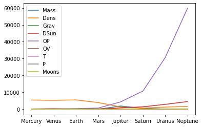
7️⃣.5️⃣ DataFrame Vizualization
Visualization communicates data trends by summarizing data graphically. It is a representation of information in the form of a plot, chart, or diagram. Visualization conveys meaning by showing a distribution, correlation, or directional trend. Use .plot to create a line plot of the data. The x-labels, y-yabels, and legend are automatically generated from the DataFrame information.
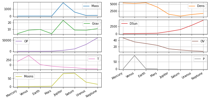
📈 Customize Plots
The plots can be adjusted to better show the information. It is typical to display each column as a separate subplot with a separate box. Options include:
- figsize - figure size
- subplots - display each column as a separate trend
- grid - display grid lines
- layout - subplot layout in rows x columns
Pandas uses matplotlib as the default backend for displaying the plots. Use pass in a Jupyter notebook to not display the plot object name.
pass
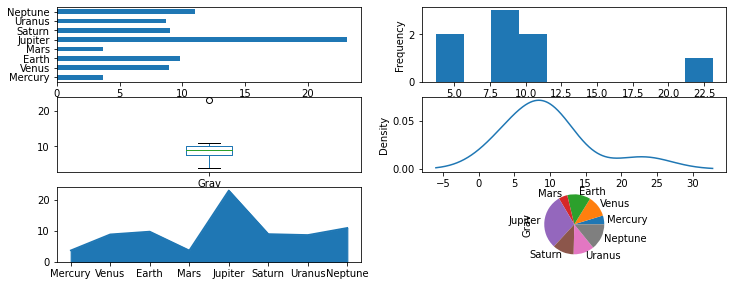
🔨 The optional parameter kind is the type of plot with the default as line.
- line : line plot (default)
- bar : vertical bar plot
- barh : horizontal bar plot
- hist : histogram
- box : boxplot
- kde / density : Kernel Density Estimation plot
- area : area plot
- pie : pie plot
- scatter : scatter plot
- hexbin : hexbin plot
A sample of the types of plots are shown below with Grav (Surface Gravity) for each planet.
t = ['barh','hist','box','kde','area','pie']
plt.figure(figsize=(12,8))
for i,ti in enumerate(t):
ax = plt.subplot(5,2,i+1)
pl['Grav'].plot(kind=ti,ax=ax)
✅ Knowledge Check: Create a bar chart (kind='bar') of the planet Mass that has a log-scale y-axis (logy=True) to see the mass of the smaller rocky planets relative to the larger gas planets.
7️⃣.6️⃣ DataFrame Export
There are many options to export a DataFrame including a data file, database, clipboard, or web-page. Some of the options to export data are for computers to efficiently transform or store the data.
pl.to_excel() - to Excel spreadsheet
pl.to_feather() - to binary Feather format for fast and compact storage
pl.to_gbq() - to Google BigQuery
pl.to_hdf() - to an HDF5 (Hierarchical Data Format) file
pl.to_json() - to a JSON file (JavaScript Object Notation)
pl.to_parquet() - to Parquet for compact data storage in Apache Hadoop
pl.to_pickle() - to Pickle file to store Python objects
pl.to_records() - to a NumPy record array
pl.to_sql() - to SQL database
pl.to_stata() - to Stata dta format
As an example, export pl to a Python dictionary.
print(pdict['Mass'])
    {'Mercury': 0.33, 'Venus': 4.87, 'Earth': 5.97,
	 'Mars': 0.642, 'Jupiter': 1898.0, 'Saturn': 568.0,
	 'Uranus': 86.8, 'Neptune': 102.0}
🗒 Human Readable Text
Other export options are intended as human-readable forms.
pl.to_csv() - to a Comma Separated Value (CSV) text file
pl.to_html() - to an HTML file (web-page)
pl.to_latex() - to LaTeX as a high-quality typesetting system
pl.to_markdown() - to Markdown for creating formatted text
pl.to_string() - to a console-friendly tabular output
Converting Mass to a string reveals a table with new-line \n characters.
    'Mercury       0.330\n
	 Venus         4.870\n
	 Earth         5.970\n
	 Mars          0.642\n
	 Jupiter    1898.000\n
	 Saturn      568.000\n
	 Uranus       86.800\n
	 Neptune     102.000'
✅ Knowledge Check: Export pl to an Excel file named planets.xlsx. Open the file with a spreadsheet application to verify that the table is exported successfully. The file is stored in the current working directory. Use os.getcwd() to show the current working directory.
print(os.getcwd())
✅ Knowledge Check
1. What is Pandas primarily used for in Python?
2. Which method is used to create a basic statistical summary of the data in a Pandas DataFrame?