Data-Driven Engineering

Data-driven engineering relies on information, often stored in the form of collections of numbers as matrices and arrays. NumPy (Numerical Python extensions) is a library for data processing with multi-dimensional arrays and mathematical functions to operate on the arrays. This series is an introduction to the Python NumPy libraries.

• 6️⃣.1️⃣ NumPy Install and Import
• 6️⃣.2️⃣ Numpy Arrays
• 6️⃣.3️⃣ Import and Export Data
• 6️⃣.4️⃣ Unary Operations
• 6️⃣.5️⃣ Binary Operations

6️⃣.1️⃣ 📒 NumPy Install and Import

Anaconda comes with numpy, scipy, and other foundational libraries. If a library is not installed, it can be added by using the name of the library with pip in a Jupyter Notebook cell or from the computer command line. Additional information on managing packages is avaiable in the Data-Driven Engineering course.

Once a library is installed, functions are imported in one of many ways:

The first option is rarely used because the full numpy name would need to be used on every function call. The second option shortens the library name and is the most popular way to import all numpy functions and attributes. The third method imports only the specific function array instead of all functions. Never use from numpy import * because it clutters the namespace and the source of the function is unclear when multiple libraries are used.

There are NumPy functions for statistical analysis, linear algebra operations, and to generate summary information. NumPy can be slower than base Python for simple operations, but is much faster for large-scale transformations. Many of the functions are written in Fortran and called from a Python interface.

• array: create a NumPy array
• hstack: join arrays along a new horizontal axis
• linspace: generate evenly spaced numbers
• max and min: maximum and minimum values
• mean: mean (average) value
• ones: generate an array of ones
• reshape: reshape an array
• sort: sort an array
• std: standard deviation
• shape: return the shape of an array
• transpose: reverse (transpose) the axes of an array
• vstack: join arrays along a new vertical axis
• zeros: generate an array of zeros

A first step in working with NumPy is to create an array. The next section demonstrates how to create a NumPy array, a fundamental data structure in the NumPy package.

6️⃣.2️⃣ 📒 NumPy Arrays

NumPy arrays are collections of number or objects stored as a vector (1D array), matrix (2D array), or multi-dimensional array (3D+ array). A tensor is a type of multi-dimensional array with certain transformation properties.

🔢 NumPy Scalar

A single number is called a scalar in NumPy. Use the np.array() function to create a new array. The input argument of the function is the array as a Python list (e.g. [7]) or tuple (e.g. (7,)).

    [7]
    <class 'numpy.ndarray'>

🔢 NumPy 1D Array

A 1-dimensional array is a row vector in NumPy.

📝 Print List and Length

Print the array with the print() function.

    [0 1 2 3 4]

The length of the array is obtained with len(y).

    5

🔢 NumPy 2D Array

A 2-dimensional array is a matrix in NumPy. The 2D array is input as a list (e.g. [0,1,2,3]). Each row list is seperated by a comma as ],[],[ to create the matrix.

    [[ 0  1  2  3]
     [10 11 12 13]
     [20 21 22 23]]
    <class 'numpy.ndarray'>

📏 The len() function returns the number of rows.

    3

⬛ Use np.size() to get the total number of array elements.

    12

📐 Use np.shape() to get the number of rows and columns as a tuple.

    (3, 4)

🔢 NumPy 3D Array

A 3-dimensional array is used for color images with pixel location horizontal position, pixel location vertical position, and color intensity (0-255) for red, green, blue (RGB). Each pixel is stored as [R,G,B] with Red=[255,0,0], Green=[0,255,0], Blue=[0,0,255], White=[255,255,255] and Black=[0,0,0]. Common image processing packages Matplotlib and Pillow use RGB while OpenCV uses the opposite order with blue first and red last (BGR).

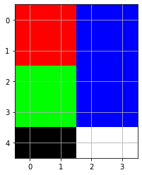
Use np.shape() to get the shape of the array with row=height (h), columns=width (w), RGB=color (c) of the image.

    5 4 3

6️⃣.3️⃣ Export and Import Data

Importing and exporting data to files is an important task for data-driven engineering. There are many methods to import and export data in Python such as the open() and close() functions in base Python. There are specialized functions to import and export large data sets in Python with Numpy, Pandas, and other packages.

One way to create a file in Numpy is with the np.save() function that saves the data in binary form (not human readable). Opening the img.npy file with a text editor has some information about the array but no human readable information about the data that is stored in compressed format.

Binary img.npy file

    “NUMPY v {'descr': '<i4', 'fortran_order':
	  False, 'shape': (8, 7, 3),}
    ÿ   ÿ   ÿ
    ÿ   ÿ  
    ÿ   ÿ  
    ÿ   ÿ  

🗄 Save Multiple Arrays

Multiple arrays can be saved to a single data zip file. Any name can be provided instead of f1, f2, or f3. These names become the key when the file is loaded.

📖 Load Data

Load the arrays with np.load() after they are saved with np.savez(). The values are available by using the name of the string key data['f3'].

    [0 1 2 3 4]

🗒 Human Readable Text Files

Save the file as a text file with np.savetxt() to create a human-readable file z.txt file.

    0.00000000e+00 1.0000000e+00 2.0000000e+00 3.00000000e+00
    1.00000000e+01 1.1000000e+01 1.2000000e+01 1.30000000e+01
    2.00000000e+01 2.1000000e+01 2.2000000e+01 2.30000000e+01

Attempting to save a higher-dimensional array than 1D or 2D produces and error: ValueError: Expected 1D or 2D array, got 3D array instead.

Switch to comma separated values (CSV versus the default tab-delimited) with delimiter=',', add a heading with header, remove # comments with comments=#, and change the format to 8 decimals with fmt='%.8e'.

    Col0,Col1,Col2
    0.00000000e+00,1.00000000e+00,2.00000000e+00,3.00000000e+00
    1.00000000e+01,1.10000000e+01,1.20000000e+01,1.30000000e+01
    2.00000000e+01,2.10000000e+01,2.20000000e+01,2.30000000e+01

Disadvantages of using text files to store data are that the file sizes are larger and the numbers may not be exactly loaded because of potential trucation.

Other common format specifiers include:

• d: signed integer
• e or E: floating point exponential format (e=lowercase, E=uppercase)
• f or F: floating point decimal format
• g or G: same as e/E if exponent is >=6 or <=-4, f otherwise
• s: string

The number 8 indicates how many decimal places are displayed.

6️⃣.4️⃣ Unary Operations

Unary operations are those performed on a single array. An example is to reverse the sign of all numbers in an array.

    array([[  0,  -1,  -2,  -3],
           [-10, -11, -12, -13],
           [-20, -21, -22, -23]])

Mathematical operations operate on the array separately for each entry. The expression 1/(z+1) is equivalent to (z+1)**-1. This is not the inverse of the matrix but only the inverse of each element in the matrix.

    array([[1.        , 0.5       , 0.33333333, 0.25      ],
           [0.09090909, 0.08333333, 0.07692308, 0.07142857],
           [0.04761905, 0.04545455, 0.04347826, 0.04166667]])

🔃 Transpose Matrix

A common unary operation is to transpose a matrix by reversing the order of the axes.

    array([[ 0, 10, 20],
           [ 1, 11, 21],
           [ 2, 12, 22],
           [ 3, 13, 23]])

🆎 Convert to Another Data Type

Convert to int, float, or str with astype() at the end of the array. There is no numerical difference with switching from an int to a float but some functions require one or the other.

    array([['0', '1', '2', '3'],
           ['10', '11', '12', '13'],
           ['20', '21', '22', '23']], dtype='<U11')

📇 Array Index

An array index refers to the location of the data. Python is zero-index so z[0,1] refers to the upper left value at row=0 and column=1.

    1

The last value has an index of -1, the second to last value has an index of -2, and so on.

    22

🔪 Array Slicing

A subset of the array is returned by slicing by indicating a range start:end instead of a single value. The slice z[0:2] returns the first two rows.

    array([[ 0,  1,  2,  3],
           [10, 11, 12, 13]])

The last two columns of any matrix are available with z[:,:-2]. A blank start or end value indicates that it should start at the beginning or proceed to the end.

    array([[ 0,  1],
           [10, 11],
           [20, 21]])

A third index refers to the step size with start:end:row_increment. Return every other row with z[0:5:2] or a shortened form with z[::2].

    array([[ 0,  1,  2,  3],
           [20, 21, 22, 23]])

Reverse the row order with z[::-1].

    array([[20, 21, 22, 23],
           [10, 11, 12, 13],
           [ 0,  1,  2,  3]])

A matrix inverse is only applicable to square matrices. This slice creates a 3x3 matrix with np.linalg.inv() calculating the inverse.

  array([[ 2.81474977e+14, -5.62949953e+14,  2.81474977e+14],
         [-5.62949953e+14,  1.12589991e+15, -5.62949953e+14],
         [ 2.81474977e+14, -5.62949953e+14,  2.81474977e+14]])

6️⃣.5️⃣ Binary Operations

Binary operations are those that involve 2 arrays. The operators available for scalars are also available for NumPy arrays.

⚙ Operators

- + - * / addition, subtraction, multiplication, division - % modulo (remainder after division) - // floor division (discard the fraction, no rounding) - ** exponential - @ matrix dot product

    array([[ 0,  2,  4,  6],
           [20, 22, 24, 26],
           [40, 42, 44, 46]])

    array([[0.        , 0.5       , 0.66666667, 0.75      ],
           [0.90909091, 0.91666667, 0.92307692, 0.92857143],
           [0.95238095, 0.95454545, 0.95652174, 0.95833333]])

🔢🔢 Array Multiplication

Array multiplication is available with the cross product np.cross() or dot product np.dot() or shortened notation @. The dot product of z.T and z is z.T@z.

    array([[500, 530, 560, 590],
           [530, 563, 596, 629],
           [560, 596, 632, 668],
           [590, 629, 668, 707]])

🧭 Comparison Operators

Comparison operators return a boolean True or False for each element of the array as a new array.

- > greater than, >= or equal to - < less than, <= or equal to - == equal to (notice the double equal sign, single assigns a value) - != or <> not equal to

    array([[False, False, False, False],
           [False,  True,  True,  True],
           [ True,  True,  True,  True]])

The np.where() command selects only the subset that are True. Use np.reshape() to get the flattened array into a desirable form, if needed.

    array([ 0,  1,  2,  3, 10])

➕ Add to Array

Items are added to an array using the np.append() function.

    array([ 0,  1,  2,  3, 10, 11, 12, 13,
	       20, 21, 22, 23,  1,  1,  1,  1])

Preserve the dimensions of the matrix by using np.vstack() for vertical stacking.

    array([[ 0,  1,  2,  3],
           [10, 11, 12, 13],
           [20, 21, 22, 23],
           [ 1,  1,  1,  1]])

Use np.hstack() for horizontal placement. Convert [-1,-1,-1] from a row vector to a column vector with np.reshape([-1,-1,-1],(-1,1)) or np.array([-1,-1,-1]).reshape(-1,1).

    array([[-1],
           [-1],
           [-1]])

    array([[ 0,  1,  2,  3, -1],
           [10, 11, 12, 13, -1],
           [20, 21, 22, 23, -1]])

💻 Exercise 6A

Create y as a 5x5 Numpy array of ones. Modify the array to place zeros along the diagonal.

💻 Exercise 6B

Create 20 uniformly distributed random numbers between 0 and 1 with np.random.rand(20)

Find the array index of the highest number with np.argmax(z)

Using the index i, print the highest number.

💻 Exercise 6C

Create 20 uniformly distributed random numbers between 0 and 1 with np.random.rand(20)

Use the np.where() function to create a new array with values from z that are greater than 0.7.

💻 Exercise 6D

Save the array z=np.random.rand(20) as a text file.

💻 Exercise 6E

Calculate the dot product of matrices A and B.

$$A = \begin{bmatrix}1 & -1\\ 5 & -7\end{bmatrix}$$

$$B = \begin{bmatrix}3 & -4\\ -2 & 2\end{bmatrix}$$

---

✅ Knowledge Check

1. Which of the following statements regarding NumPy is correct?

2. When working with NumPy arrays, how can you obtain the number of rows in a 2D array (e.g. array = np.ones((3,2)) as an array of ones with three rows and two columns)?