Audio Data Analysis


Audio data and analysis are transforming how computers interact with people and provide useful services. Digital assistants use Natural Language Processing (NLP) that is driven by machine learning to translate audio signals into text. Audio data is used to detect intrusion, anticipate rotating equipment failure such as in pumps and turbines, and acoustic location of firearm discharge in cities. This tutorial is a demonstration of audio data analysis with an application to detect a nearby drone.
Import Audio Libraries
The first step is to import libraries for audio analysis. Numpy, Scipy, and Matplotlib are standard libraries in Python. An additional library is pydub (to convert stereo to mono) that can be installed with pip install pydub. See information on how to Install Python Packages.
import matplotlib.pyplot as plt
from scipy.io import wavfile
from scipy import signal
from pydub import AudioSegment
Download Audio File
Download Drone1.wav or use the script to download the file to the run directory.
f = 'Drone1.wav' # or Drone2.wav, Drone3.wav
url = 'http://apmonitor.com/dde/uploads/Main/'+f
urllib.request.urlretrieve(url,f)
Import Audio File
Once the required packages are imported, the audio file Drone1.wav is imported. A wav file is not a compressed storage form such as mp3 files that typically require much less (typically 5x) storage for similar audio quality.
f = 'Drone1.wav'
#s = sampling (int)
#a = audio signal (numpy array)
s,a = wavfile.read(f)
print('Sampling Rate:',s)
print('Audio Shape:',np.shape(a))
    Sampling Rate: 48000
    Audio Shape: (387072, 2)
The sampling rate is 48 kHz and there are 2 channels with 387,072 total sample points for a total of 387072/48000 = 8.064 sec.
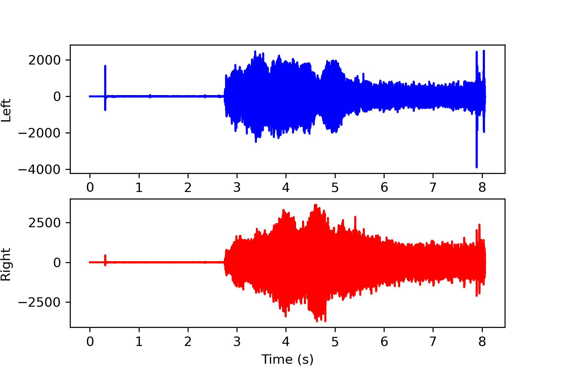
Display Original Signal
Display the magnitude of the original sound from the 2 channels (stereo). Stereo contains two audio streams that are synchronized to create surround sound in 2 dimensions.
na = a.shape[0]
#audio time duration
la = na / s
#plot signal versus time
t = np.linspace(0,la,na)
plt.subplot(2,1,1)
plt.plot(t,a[:,0],'b-')
plt.ylabel('Left')
plt.subplot(2,1,2)
plt.plot(t,a[:,1],'r-')
plt.ylabel('Right')
plt.xlabel('Time (s)')
plt.show()
Convert to One Channel (Stereo to Mono)
Several audio analysis packages require a single audio stream (mono) for analysis. The pydub package can be used to set the number of channels to 1 and export as a new audio file with _mono.wav appended to the end of the file name. The f[:-4] code removes the last 4 characters of the file name .wav.
sound = sound.set_channels(1)
fm = f[:-4]+'_mono.wav'
sound.export(fm,format="wav")
Import Audio File
Humans can perceive sound in the range of 20 Hz to 20 kHz. Ultrasound has a frequency higher than the upper human auditory limit of 20 kHz. Common sampling rates are 44.1 kHz and 48 kHz. Higher sampling rates (88.2 kHz, 96 kHz and 192 kHz) are also common in music production. Medical ultrasound machines use waves with a frequency ranging between 2 and 15 MHz. Import the new single channel audio file with sampling rate 48 kHz.
print('Sampling Rate:',s)
print('Audio Shape:',np.shape(a))
    Sampling Rate: 48000
    Audio Shape: (387072,)
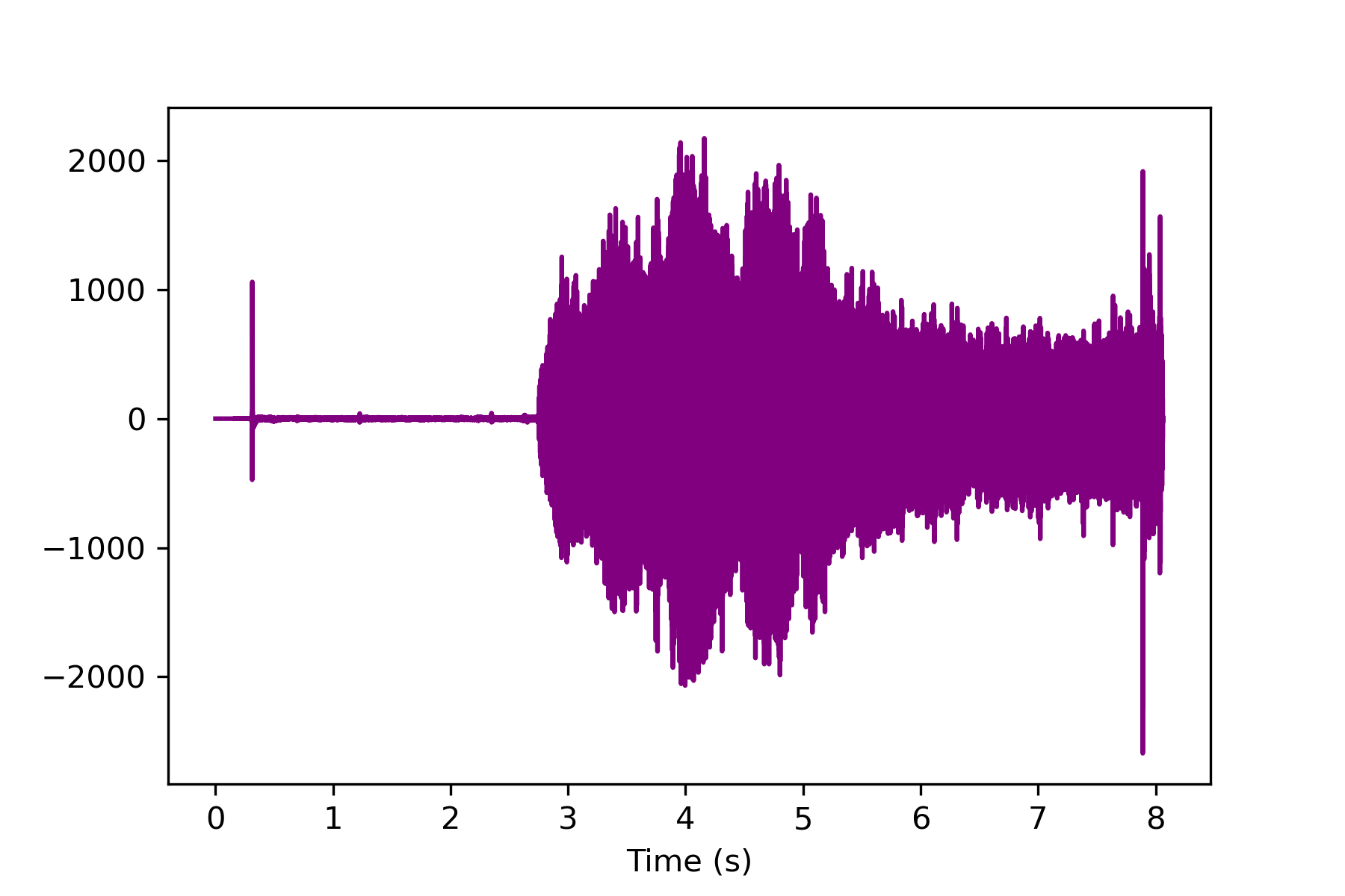
Display Modified Audio
A single channel is now available for analysis. The audio magnitude grows as the drone is turned on and begins flying nearby.
la = na / s
t = np.linspace(0,la,na)
plt.plot(t,a,'k-',color='purple')
plt.xlabel('Time (s)')
plt.show()
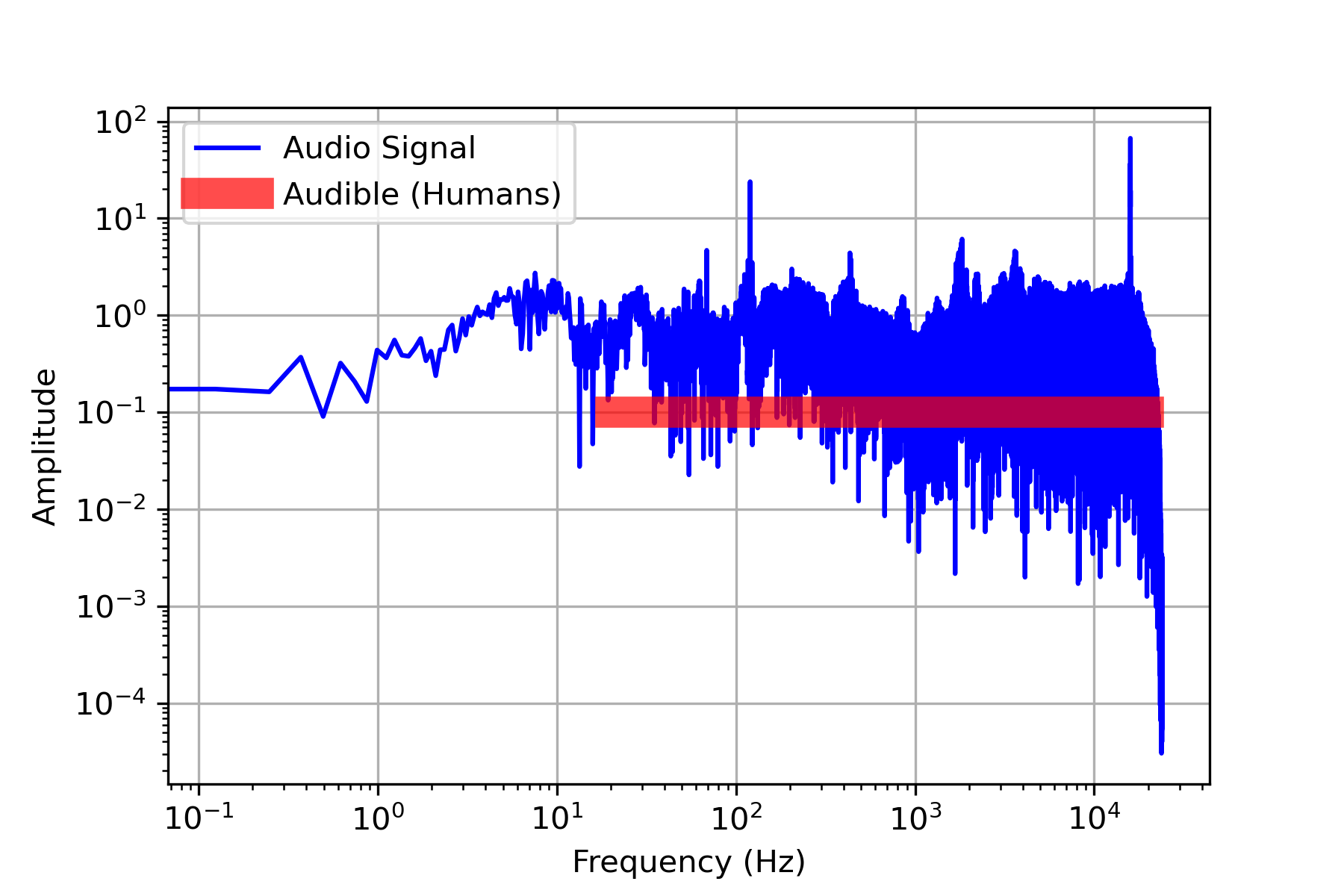
Frequency Analysis
A Fast Fourier Transform (FFT) analysis shows the frequency content of the entire 8 second audio file.
na = len(a)
a_k = np.fft.fft(a)[0:int(na/2)]/na # FFT function from numpy
a_k[1:] = 2*a_k[1:] # single-sided spectrum only
Pxx = np.abs(a_k) # remove imaginary part
f = s*np.arange((na/2))/na # frequency vector
#plotting
fig,ax = plt.subplots()
plt.plot(f,Pxx,'b-',label='Audio Signal')
plt.plot([20,20000],[0.1,0.1],'r-',alpha=0.7,\
linewidth=10,label='Audible (Humans)')
ax.set_xscale('log'); ax.set_yscale('log')
plt.grid(); plt.legend()
plt.ylabel('Amplitude')
plt.xlabel('Frequency (Hz)')
plt.show()
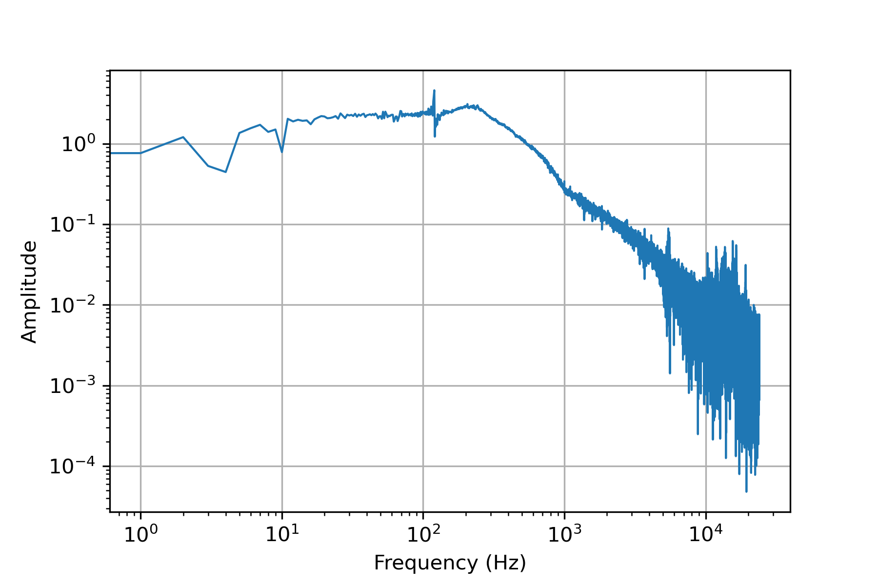
A segment of 48000 samples (1 sec) is analyzed for frequency content. The first second has the beep of the drone controller turning on and connecting to the drone. Otherwise, it is relatively quiet during the first second of audio.
na = s
a_k = np.fft.fft(a[:na])[0:int(na/2)]/na # FFT function from numpy
a_k[1:] = 2*a_k[1:] # single-sided spectrum only
Pxx = np.abs(a_k) # remove imaginary part
f = s*np.arange((na/2))/na # frequency vector
#plotting
fig,ax = plt.subplots()
plt.plot(f,Pxx,linewidth=1)
ax.set_xscale('log'); ax.set_yscale('log')
plt.ylabel('Amplitude'); plt.grid()
plt.xlabel('Frequency (Hz)')
plt.show()
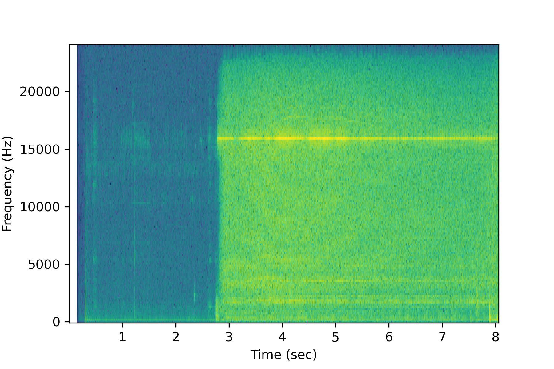
Spectrogram
A spectrogram displays the frequency power at each time segment. The natural log of the spectrogram improves the visibility of the frequency content so that a few large peaks do not remove the resolution of the entire spectrogram.
lspg = np.log(spgram)
plt.pcolormesh(tm,fr,lspg,shading='auto')
plt.ylabel('Frequency (Hz)')
plt.xlabel('Time (sec)')
plt.show()
Features for Machine Learning
Now that the audio data is imported and analyzed for frequency content, it may be desireable to create features for machine learning regression or classification. All frequencies within the auditory range (20 Hz-20 kHz) may be too many.
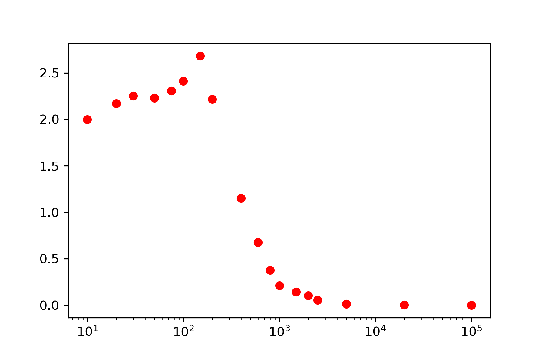
Bin the Frequencies
A clustering approach uses bins to aggregate the frequency power between specified limits.
fb = np.array([0,10,20,30,50,75,100,150,200,400,600,\
800,1000,1500,2000,2500,5000,20000,100000])
Pb = np.zeros(len(fb))
nb = np.zeros(len(fb))
ibin = 0
n = 0
for i in range(len(f)):
if f[i]>fb[ibin+1]:
ibin+=1
nb[ibin]+=1
Pb[ibin]+=Pxx[i]
for i in range(len(fb)):
if nb[i] == 0:
nb[i]=1
Pb[i] = Pb[i]/nb[i]
fig,ax = plt.subplots()
plt.semilogx(fb,Pb,'ro',linewidth=1)
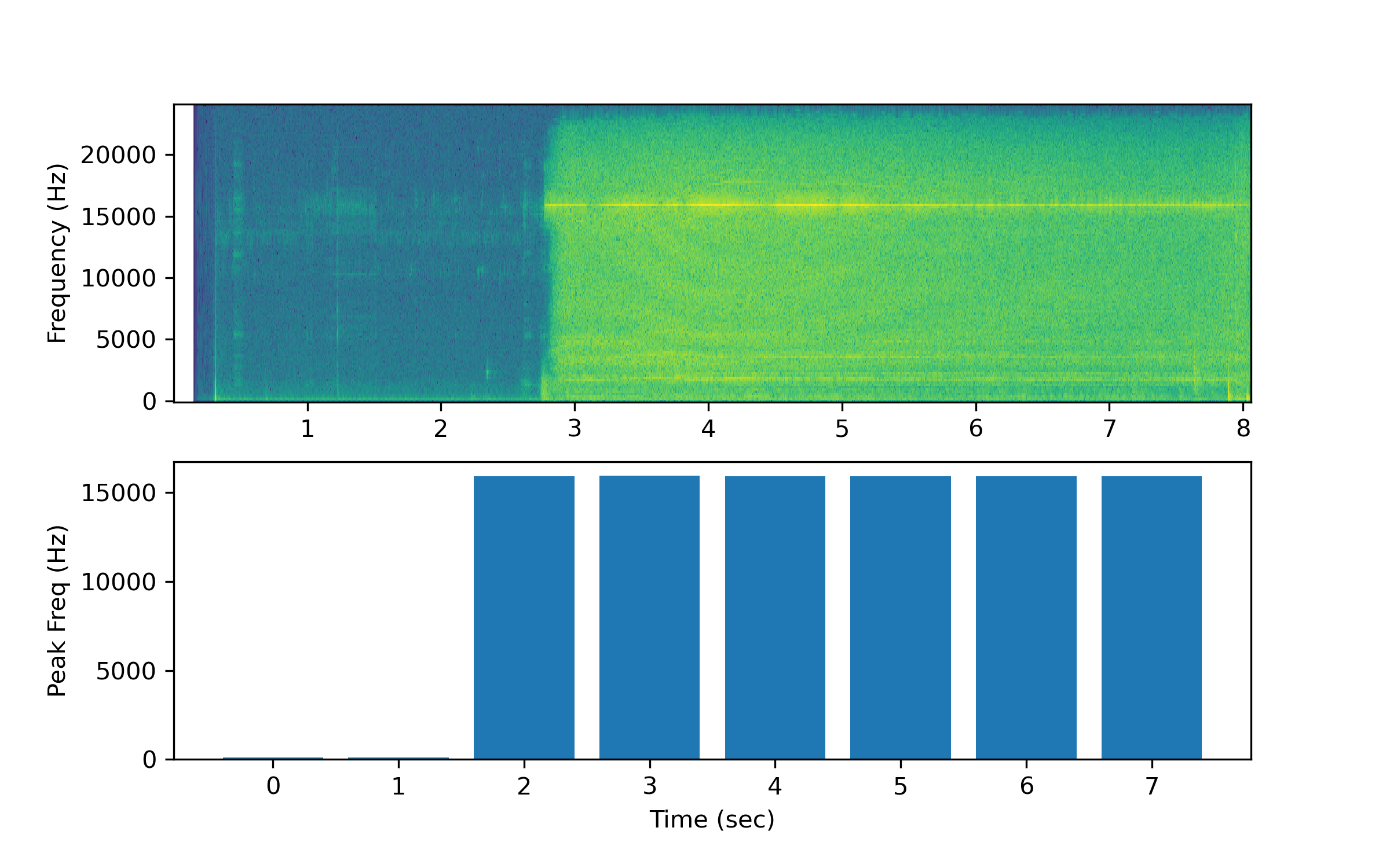
Peak Frequency
nsec = int(np.floor(la))
pf = np.empty(nsec)
for i in range(nsec):
audio = a[i*s:(i+1)*s]; na=len(audio) # use 48000 points with 48kHz
a_k = np.fft.fft(audio)[0:int(na/2)]/na
a_k[1:] = 2*a_k[1:]
Pxx = np.abs(a_k)
f = s*np.arange((na/2))/na
ipf = np.argmax(Pxx)
pf[i] = f[ipf]
plt.figure(figsize=(8,5))
plt.subplot(2,1,1)
plt.pcolormesh(tm,fr,lspg,shading='auto')
plt.ylabel('Frequency (Hz)')
plt.subplot(2,1,2)
tb = np.arange(0,nsec)
plt.bar(tb,pf)
plt.xlabel('Time (sec)'); plt.ylabel('Peak Freq (Hz)')
plt.show()
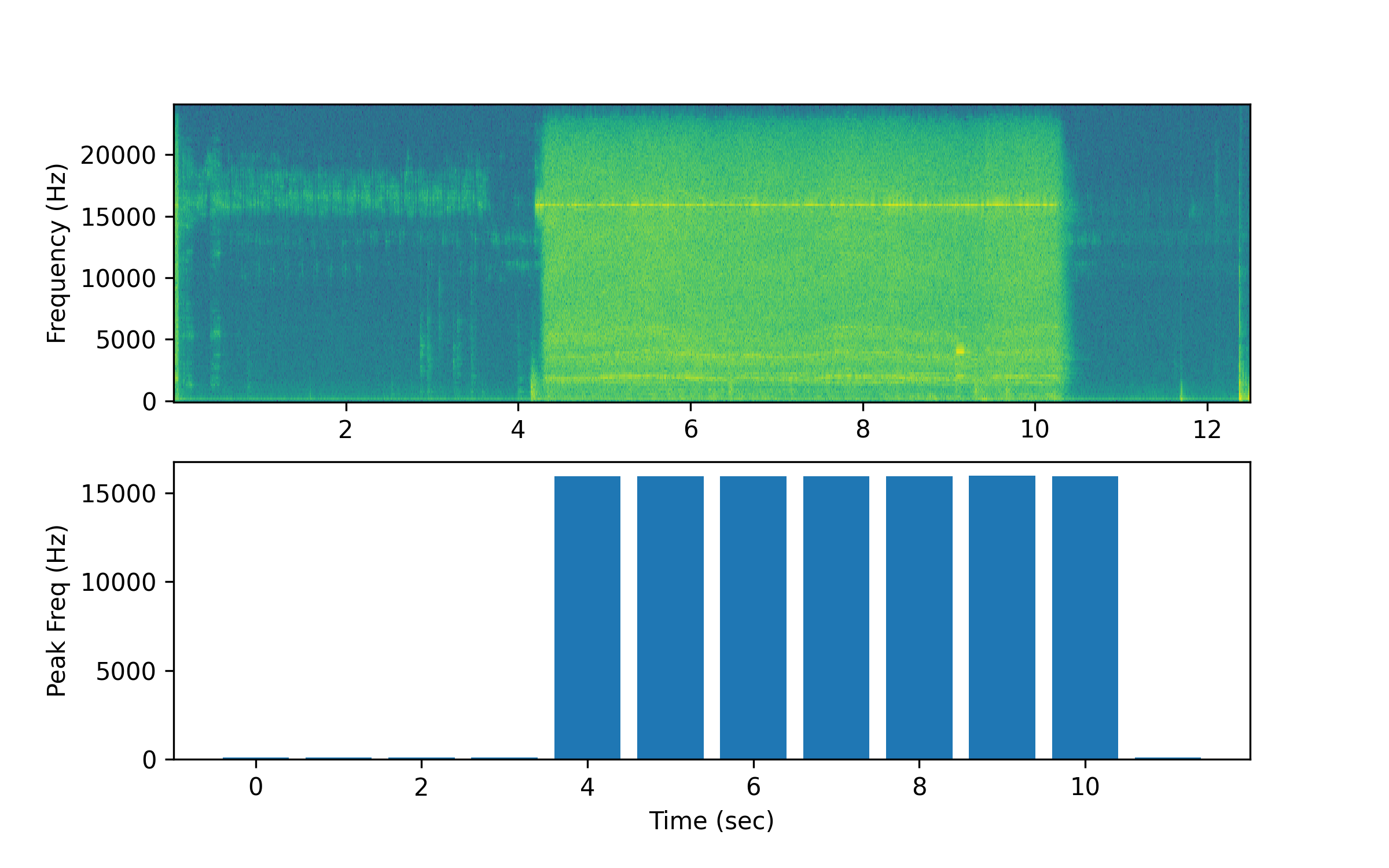
Activity

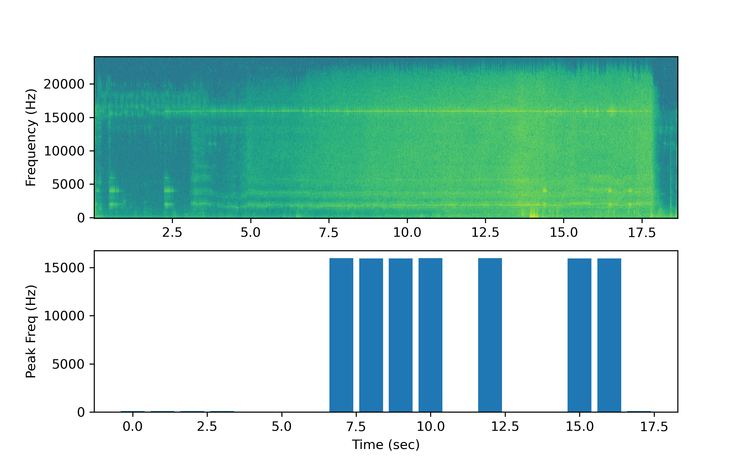
Analyze two additional audio samples to detect the presence of a drone. The first of two (Drone2.wav) is a relatively easy case where the drone takes off and lands within the audio segment. Analyze Drone2.wav by modifying the notebook and replacing Drone1.wav with Drone2.wav.

import matplotlib.pyplot as plt
from scipy.io import wavfile
from scipy import signal
import urllib.request
from pydub import AudioSegment
f = 'Drone2.wav'
url = 'http://apmonitor.com/dde/uploads/Main/'+f
urllib.request.urlretrieve(url,f)
sound = AudioSegment.from_wav(f)
sound = sound.set_channels(1)
fm = f[:-4]+'_mono.wav'
sound.export(fm,format="wav")
s,a = wavfile.read(fm)
print('Sampling Rate:',s)
print('Audio Shape:',np.shape(a))
na = a.shape[0]
la = na / s
t = np.linspace(0,la,na)
# analyze each sec of audio clip
nsec = int(np.floor(la))
pf = np.empty(nsec)
for i in range(nsec):
audio = a[i*s:(i+1)*s]; na=len(audio) # use 48000 points with 48kHz
a_k = np.fft.fft(audio)[0:int(na/2)]/na
a_k[1:] = 2*a_k[1:]
Pxx = np.abs(a_k)
f = s*np.arange((na/2))/na
ipf = np.argmax(Pxx)
pf[i] = f[ipf]
fr, tm, spgram = signal.spectrogram(a,s)
lspg = np.log(spgram)
plt.figure(figsize=(8,5))
plt.subplot(2,1,1)
plt.pcolormesh(tm,fr,lspg,shading='auto')
plt.ylabel('Frequency (Hz)')
plt.subplot(2,1,2)
tb = np.arange(0,nsec)
plt.bar(tb,pf)
plt.xlabel('Time (sec)'); plt.ylabel('Peak Freq (Hz)')
plt.savefig('drone2.png',dpi=300)
plt.show()
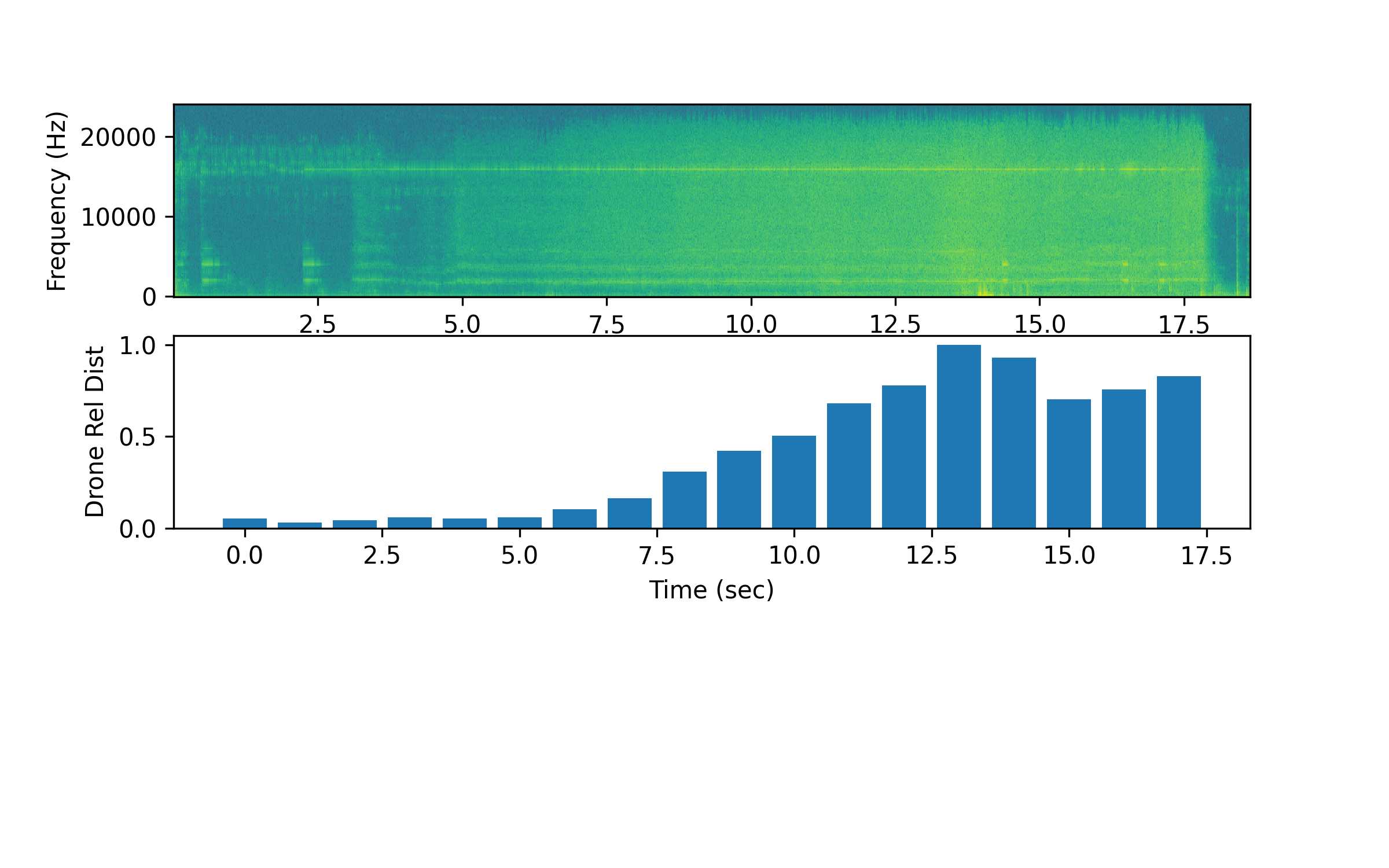
In the second case (Drone3.wav), the drone takes off from far away and moves closer. How could the program be modified to improve the drone detection as it approaches?
The detection program using only the peak frequency does not perform well for this case. Modify the detection algorithm to improve identification of the drone audio signature. A possible method is to analyze the power in the known frequency of the drone or build features to train and predict with a classifier.
A potential classification approach is to use a Convolutional Neural Network (CNN) of the spectrogram image to decide if there is a drone or no drone nearby. See the related Concrete Crack Classification with CNNs.
There isn't enough data to train a classifier. A classifier typically needs a minimum of 30 samples before Machine Learning is possible and some algorithms such as Neural Networks can require many more labeled samples.
One potential solution is to isolate the signal power in the 15,000 to 16,000 Hz range. A summation of the audio power level in this region is used to create an estimate of the relative distance to the drone.
Additional data on drone position with the audio is needed to estimate an absolute distance to the drone. A cutoff distance (or audio power level) could be used to detect whether a drone is nearby.
import matplotlib.pyplot as plt
from scipy.io import wavfile
from scipy import signal
import urllib.request
from pydub import AudioSegment
f = 'Drone3.wav'
url = 'http://apmonitor.com/dde/uploads/Main/'+f
urllib.request.urlretrieve(url,f)
sound = AudioSegment.from_wav(f)
sound = sound.set_channels(1)
fm = f[:-4]+'_mono.wav'
sound.export(fm,format="wav")
s,a = wavfile.read(fm)
print('Sampling Rate:',s)
print('Audio Shape:',np.shape(a))
na = a.shape[0]
la = na / s
t = np.linspace(0,la,na)
# analyze each sec of audio clip
nsec = int(np.floor(la))
pf = np.empty(nsec)
for i in range(nsec):
audio = a[i*s:(i+1)*s]; na=len(audio) # use 48000 points with 48kHz
a_k = np.fft.fft(audio)[0:int(na/2)]/na
a_k[1:] = 2*a_k[1:]
Pxx = np.abs(a_k)
f = s*np.arange((na/2))/na
pf[i] = np.sum(Pxx[np.where((f>15000)&(f<=16000))])
# normalize
pf = pf / np.max(pf)
fr, tm, spgram = signal.spectrogram(a,s)
lspg = np.log(spgram)
plt.figure(figsize=(8,5))
plt.subplot(3,1,1)
plt.pcolormesh(tm,fr,lspg,shading='auto')
plt.ylabel('Frequency (Hz)')
plt.subplot(3,1,2)
tb = np.arange(0,nsec)
plt.bar(tb,pf)
plt.xlabel('Time (sec)'); plt.ylabel('Drone Rel Dist')
plt.savefig('drone3.png',dpi=300)
plt.show()

✅ Knowledge Check
1. What is the main purpose of audio data analysis activity?
- Incorrect. While the tutorial does convert audio signals into visual representations like plots and graphs, the main purpose of this tutorial is to demonstrate audio data analysis with an application to detect a nearby drone.
- Incorrect. The tutorial does not focus on playing back audio signals, but rather on analyzing them to detect drones.
- Correct. This is the main purpose of the given tutorial on audio data analysis.
- Incorrect. Although the content mentions that digital assistants use audio signals, the main focus of the tutorial is on drone detection.
2. What is the function of the pydub library in the audio analysis process?
- Incorrect. FFT is used to analyze the frequency content of the audio signal, and this is not the primary function of the pydub library.
- Correct. The pydub library is used in the tutorial to convert stereo audio files into a single channel (mono) audio file.
- Incorrect. The urllib.request library is used to download the audio files, not pydub.
- Incorrect. The pydub library is not used for playback in the tutorial; it's used for audio file conversion.