Dynamics and Control

Objective: Linearize and simulate an energy balance model with radiative and convective heat transfer.

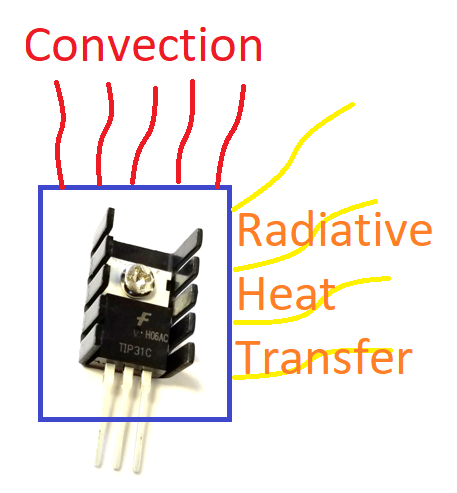
An energy balance equation includes convective and radiative heat transfer and is nonlinear because of the T⁴ term.

$$\frac{dT}{dt} = f(T,Q) = \frac{U\,A\, \left(T_a-T\right) + \epsilon\,\sigma\,A\,\left(T_\infty^4-T^4\right) + \alpha \, Q}{m \, c_p}$$

Linearize the nonlinear differential equation by computing the partial derivatives `\gamma` and `\beta` with respect to the heater value (Q) and temperature (T). The `\gamma` and `\beta` are constants when evaluated at steady state conditions. The right hand side of the differential equation is a function f(T,Q) of only Q and T while the other values are constants.

$$\frac{dT}{dt} = \frac{\partial f}{\partial T}\bigg|_{\bar T,\bar Q} \left(T-\bar T\right) + \frac{\partial f}{\partial Q}\bigg|_{\bar T,\bar Q} \left(Q-\bar Q\right)$$

Condensed Linear Form

$$\frac{dT'}{dt} = \gamma T' + \beta Q'$$

with partial derivatives evaluated at steady state conditions (`\bar Q`=0, `\bar T`=23^oC):

$$\gamma = \frac{\partial f}{\partial T}\bigg|_{\bar T,\bar Q}$$

$$\beta = \frac{\partial f}{\partial Q}\bigg|_{\bar T,\bar Q}$$

and deviation variables as the difference from the steady state conditions:

$$T' = T - \bar T$$

$$Q' = Q - \bar Q$$

Use values `\alpha`=0.01, `T_a`=23^oC, m=0.004 kg, `\epsilon`=0.9, A=0.0012 m², `c_p`=500 J/kg-K, U=5 W/m²-K, `\sigma`=5.67x10^-8 W/m²-K⁴ , and `T_\infty`=23 ^oC to simulate the change in temperature over the 5 minutes when heater Q is adjusted to 75%. Compare the simulated temperature response to data from the TCLab as well as the nonlinear model. Add the linear simulation prediction to the solution from the prior TCLab exercise.

Add Linear Simulation and Connect TCLab to Add Data to Plot

import numpy as np
import matplotlib.pyplot as plt
from scipy.integrate import odeint
import tclab
import time

n = 300  # Number of second time points (5 min)

# collect data if TCLab is connected
try:
    lab = tclab.TCLab()
    T1 = [lab.T1]
    lab.Q1(75)
    for i in range(n):
        time.sleep(1)
        print(lab.T1)
        T1.append(lab.T1)
    lab.close()
    connected = True
except:
    print('Connect TCLab to Get Data')
    connected = False

# simulation
U = 5.0
A = 0.0012
alpha = 0.01
eps = 0.9
sigma = 5.67e-8
Ta = 23
Cp = 500
m = 0.004
TaK = Ta + 273.15
def labsim(TC,t):
    TK = TC + 273.15
    dTCdt = (U*A*(Ta-TC) + sigma*eps*A*(TaK**4-TK**4) + alpha*50)/(m*Cp)
    return dTCdt

tm = np.linspace(0,n,n+1) # Time values
Tsim = odeint(labsim,23,tm)

# calculate losses from conv and rad
conv = U*A*(Ta-Tsim)
rad = sigma*eps*A*(TaK**4-(Tsim+273.15)**4)
loss = conv+rad
gain = alpha*50

# Plot results
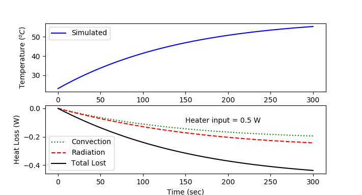
plt.figure()
plt.subplot(2,1,1)
plt.plot(tm,Tsim,'b-',label='Simulated')
if connected:
    plt.plot(tm,T1,'r.',label='Measured')
plt.ylabel(r'Temperature ($^oC$)')
plt.legend()
plt.subplot(2,1,2)
plt.plot(tm,conv,'g:',label='Convection')
plt.plot(tm,rad,'r--',label='Radiation')
plt.plot(tm,loss,'k-',label='Total Lost')
plt.text(150,-0.1,'Heater input = '+str(gain)+' W')
plt.ylabel(r'Heat Loss (W)')
plt.legend(loc=3)
plt.xlabel('Time (sec)')
plt.show()

[$[Get Code]]

Add Linear Simulation and Connect TCLab to Add Data to Plot

import numpy as np
import matplotlib.pyplot as plt
import tclab
import time
# pip install gekko
from gekko import GEKKO

n = 300  # Number of second time points (5 min)

# collect data if TCLab is connected
try:
    lab = tclab.TCLab()
    T1 = [lab.T1]
    lab.Q1(75)
    for i in range(n):
        time.sleep(1)
        print(lab.T1)
        T1.append(lab.T1)
    lab.close()
    connected = True
except:
    print('Connect TCLab to Get Data')
    connected = False

# simulation
m = GEKKO()
m.time = np.linspace(0,n,n+1)
U = 5.0; A = 0.0012; Cp = 500
mass = 0.004; alpha = 0.01; Ta = 23
eps = 0.9; sigma = 5.67e-8; TaK = Ta+273.15
TC = m.Var(Ta)
TK = m.Intermediate(TC+273.15)
conv = m.Intermediate(U*A*(Ta-TC))
rad  = m.Intermediate(sigma*eps*A*(TaK**4-TK**4))
loss = m.Intermediate(conv + rad)
gain = m.Intermediate(alpha*50)
m.Equation(mass*Cp*TC.dt()==conv+rad+gain)
m.options.NODES = 3
m.options.IMODE = 4 # dynamic simulation
m.solve(disp=False)

# Plot results
plt.figure()
plt.subplot(2,1,1)
plt.plot(m.time,TC,'b-',label='Simulated')
if connected:
    plt.plot(m.time,T1,'r.',label='Measured')
plt.ylabel(r'Temperature ($^oC$)')
plt.legend()
plt.subplot(2,1,2)
plt.plot(m.time,conv,'g:',label='Convection')
plt.plot(m.time,rad,'r--',label='Radiation')
plt.plot(m.time,loss,'k-',label='Total Lost')
plt.text(150,-0.1,'Heater input = '+str(gain.value[0])+' W')
plt.ylabel(r'Heat Loss (W)')
plt.legend(loc=3)
plt.xlabel('Time (sec)')
plt.show()

[$[Get Code]]

Solution