Automobile Velocity Control
 |  |  |  |
|---|
A self-driving car company has requested a speed controller for their new model of electric autonomous vehicles. Unlike standard cruise control systems, this speed controller must manage transitions between all velocities ranging from 0 to 25 m/s (56 mph or 90 km/hr).
The speed controller changes a gas pedal (%) input that adjusts electrical current to the motor, creates a torque on the drive train, applies forward thrust from wheel contact on the road, and changes the velocity of the vehicle. Regenerative braking is part of this application by allowing the gas pedal to go from -50% to 100%. Decreases in velocity are also due to resistive forces. Negative velocities (backwards driving) is highly undesirable.
Momentum Balance
A momentum balance is the accumulation of momentum for a control volume equal to the sum of forces F acting on the automobile.
$$\frac{d(m\,v)}{dt} = \sum F$$
with m as the mass in the vehicle and passengers and v as the velocity of the automobile. Assuming constant mass of the vehicle, a constant drag coefficient, Cd, and a linear gain between gas pedal position and force, the momentum balance becomes
$$m\frac{dv(t)}{dt} = F_p u(t) - \frac{1}{2} \rho \, A \, C_d v(t)^2 $$
with u(t) as gas pedal position (%pedal), v(t) as velocity (m/s), m as the mass of the vehicle (500 kg) plus the mass of the passengers and cargo (200 kg), Cd as the drag coefficient (0.24), `\rho` as the air density (1.225 kg/m3), A as the vehicle cross-sectional area (5 m2), and Fp as the thrust parameter (30 N/%pedal).
Control System Design
A first step in controller design is to list the PV (process variable), OP (controller output), SP (controller set point), and any potential DVs (disturbance variables). The three elements that create feedback control are a sensor, actuator, and controller.
| Element | Cruise Control |
| OP: Actuator | Gas Pedal Position |
| CV: Controller Set Point | Desired Speed (mph or km/hr) |
| PV: Measurement (Sensor) | Speedometer, measured velocity |
| DV: Disturbance variables | Hills, wind, cargo + passenger load |
Fit to First-Order Model
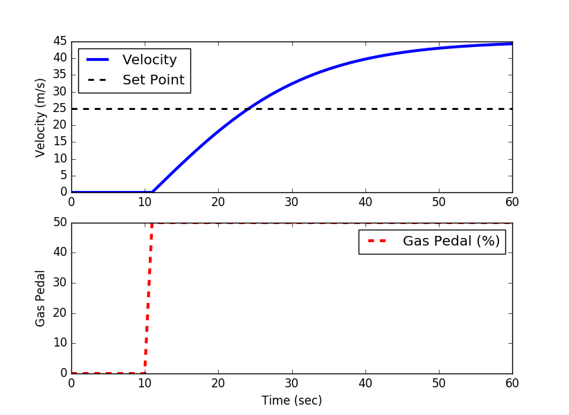
A first step in determining acceptable PID tuning parameters is to approximate the system response with a first-order plus dead-time (FOPDT) model. This can either be done approximately with graphical methods and a step response or more precisely with optimization. In this case, use the step response obtained from the simulation above to obtain parameters `K_p`, `\tau_p`, and `\theta_p`.


import matplotlib.pyplot as plt
from scipy.integrate import odeint
# animate plots?
animate=True # True / False
# define model
def vehicle(v,t,u,load):
# inputs
# v = vehicle velocity (m/s)
# t = time (sec)
# u = gas pedal position (-50% to 100%)
# load = passenger load + cargo (kg)
Cd = 0.24 # drag coefficient
rho = 1.225 # air density (kg/m^3)
A = 5.0 # cross-sectional area (m^2)
Fp = 30 # thrust parameter (N/%pedal)
m = 500 # vehicle mass (kg)
# calculate derivative of the velocity
dv_dt = (1.0/(m+load)) * (Fp*u - 0.5*rho*Cd*A*v**2)
return dv_dt
tf = 60.0 # final time for simulation
nsteps = 61 # number of time steps
delta_t = tf/(nsteps-1) # how long is each time step?
ts = np.linspace(0,tf,nsteps) # linearly spaced time vector
# simulate step test operation
step = np.zeros(nsteps) # u = valve % open
step[11:] = 50.0 # step up pedal position
# passenger(s) + cargo load
load = 200.0 # kg
# velocity initial condition
v0 = 0.0
# set point
sp = 25.0
# for storing the results
vs = np.zeros(nsteps)
sps = np.zeros(nsteps)
plt.figure(1,figsize=(5,4))
if animate:
plt.ion()
plt.show()
# simulate with ODEINT
for i in range(nsteps-1):
u = step[i]
# clip inputs to -50% to 100%
if u >= 100.0:
u = 100.0
if u <= -50.0:
u = -50.0
v = odeint(vehicle,v0,[0,delta_t],args=(u,load))
v0 = v[-1] # take the last value
vs[i+1] = v0 # store the velocity for plotting
sps[i+1] = sp
# plot results
if animate:
plt.clf()
plt.subplot(2,1,1)
plt.plot(ts[0:i+1],vs[0:i+1],'b-',linewidth=3)
plt.plot(ts[0:i+1],sps[0:i+1],'k--',linewidth=2)
plt.ylabel('Velocity (m/s)')
plt.legend(['Velocity','Set Point'],loc=2)
plt.subplot(2,1,2)
plt.plot(ts[0:i+1],step[0:i+1],'r--',linewidth=3)
plt.ylabel('Gas Pedal')
plt.legend(['Gas Pedal (%)'])
plt.xlabel('Time (sec)')
plt.pause(0.1)
if not animate:
# plot results
plt.subplot(2,1,1)
plt.plot(ts,vs,'b-',linewidth=3)
plt.plot(ts,sps,'k--',linewidth=2)
plt.ylabel('Velocity (m/s)')
plt.legend(['Velocity','Set Point'],loc=2)
plt.subplot(2,1,2)
plt.plot(ts,step,'r--',linewidth=3)
plt.ylabel('Gas Pedal')
plt.legend(['Gas Pedal (%)'])
plt.xlabel('Time (sec)')
plt.show()
Problem Statement
Design a controller that will achieve satisfactory performance in set point tracking over the range of requested driving velocities. Use physics-based modeling to create a suitable dynamic representation of the relationship between gas pedal position (%) and vehicle velocity. Create simulated step tests to fit to a first-order plus dead-time (FOPDT) model. Use the FOPDT model parameters `K_p`, `\tau_p`, and `\theta_p` to design a PI controller with parameters `K_c` and `\tau_I` (derivative time constant is zero, `\tau_D=0`). Test the controller over a range of set point changes that may be encountered in typical driving conditions. Show plots of the velocity and gas pedal position as the car achieves the desired velocity set points. Discuss how disturbances such as wind or a hill would affect the velocity and how the controller would respond.