Liquid Level Control
 |  |  |
|---|
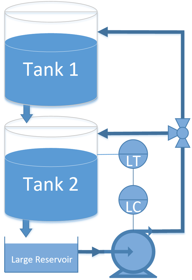
Liquid level control is important to not overfill or underfill vessels. Underfilling can damage downstream pumps by draining all liquid and continuing to operate with gas. Overfilling causes overflow of the vessel and possible loss of containment or diverting product to the flare. Startup and shutdown are transient operations that require attention to maintain appropriate levels as shown by the Texas City Refinery incident.
The objective of this case study is to automatically maintain a liquid level in the lower of two dual gravity drained tanks.
Run the Python app with streamlit. A browser window opens with the app interface.
streamlit run app_2tank_pid.py
The tasks of this exercise include:
- Create a dynamic first-order model
- Obtain PID tuning parameters
- Adjust the PID tuning with quantified performance
- Avoid overfilling tank 1 with setpoint changes to tank 2 level

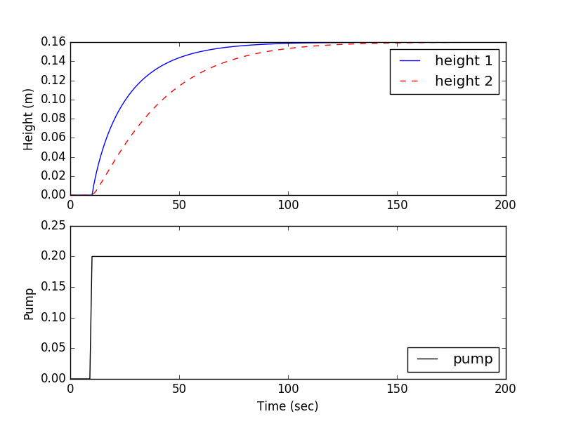
Step Test with Graphical FOPDT Fit
For the gravity drained tank problem, conduct a step test by manipulating the pump rate and recording the level in the bottom tank. Use graphical methods to obtain a FOPDT model and report the values of the three parameters `(K_p, \tau_p, \theta_p)`.
import matplotlib.pyplot as plt
from scipy.integrate import odeint
# animate plots?
animate=True # True / False
def tank(levels,t,pump,valve):
h1 = max(0.0,levels[0])
h2 = max(0.0,levels[1])
c1 = 0.08 # inlet valve coefficient
c2 = 0.04 # tank outlet coefficient
dhdt1 = c1 * (1.0-valve) * pump - c2 * np.sqrt(h1)
dhdt2 = c1 * valve * pump + c2 * np.sqrt(h1) - c2 * np.sqrt(h2)
# overflow conditions
if h1>=1.0 and dhdt1>0.0:
dhdt1 = 0
if h2>=1.0 and dhdt2>0.0:
dhdt2 = 0
dhdt = [dhdt1,dhdt2]
return dhdt
# Initial conditions (levels)
h0 = [0.0,0.0]
# Time points to report the solution
tf = 200
t = np.linspace(0,tf,tf+1)
# Inputs that can be adjusted
pump = np.zeros((tf+1))
# pump can operate between 0 and 1
pump[10:] = 0.2
# valve = 0, directly into top tank
# valve = 1, directly into bottom tank
valve = 0.0
# Record the solution
y = np.empty((tf+1,2))
y[0,:] = h0
plt.figure(1)
if animate:
plt.ion()
plt.show()
# Simulate the tank step test
for i in range(tf):
# Specify the pump and valve
inputs = (pump[i],valve)
# Integrate the model
h = odeint(tank,h0,[0,1],inputs)
# Record the result
y[i+1,:] = h[-1,:]
# Reset the initial condition
h0 = h[-1,:]
# plot results
if animate:
plt.clf()
plt.subplot(2,1,1)
plt.plot(t[0:i+1],y[0:i+1,0],'b-',label='height 1')
plt.plot(t[0:i+1],y[0:i+1,1],'r--',label='height 2')
plt.ylabel('Height (m)')
plt.legend(loc='best')
plt.subplot(2,1,2)
plt.plot(t[0:i+1],pump[0:i+1],'k-',label='pump')
plt.legend(loc='best')
plt.ylabel('Pump')
plt.xlabel('Time (sec)')
plt.pause(0.01)
# Export step test data file
# reshape as column vectors
time_col = t.reshape(-1,1)
pump_col = pump.reshape(-1,1)
h2_col = y[:,1].reshape(-1,1)
my_data = np.concatenate((time_col,pump_col,h2_col), axis=1)
np.savetxt('step_test_data.txt',my_data,delimiter=',')
if not animate:
# Plot results
plt.subplot(2,1,1)
plt.plot(t,y[:,0],'b-',label='height 1')
plt.plot(t,y[:,1],'r--',label='height 2')
plt.ylabel('Height (m)')
plt.legend(loc='best')
plt.subplot(2,1,2)
plt.plot(t,pump,'k-',label='pump')
plt.legend(loc='best')
plt.ylabel('Pump')
plt.xlabel('Time (sec)')
plt.show()
Fit FOPDT with Optimization
Use optimization to obtain the same parameters in the FOPDT model (see example optimization code). Compare the optimized values with those obtained graphically. Are they the same? Why or why not? Which values would you use and why?
Repeat with Doublet Test
Repeat the test using a doublet test instead of a step test. Fit FOPDT parameters using optimization of the three parameters `(K_p, \tau_p, \theta_p)`. Why is it important to obtain values above and below the steady state value for nonlinear processes?
Design and Tune PI Controller
Use an appropriate tuning rule (either ITAE or IMC) to obtain a starting value for the controller gain `(Kc)` and integral reset time `(\tau_I)` of a PI controller. Implement the PI controller (with anti-reset windup) and tune the controller constants (adjust up or down) until an acceptable response is achieved for step changes in the set point. Include plots of with initial values, tuned values, and a justification of your criteria for an acceptable response. Remember to define your criteria in terms of rise time, peak time, overshoot ratio, decay ratio and settling time. See Second Order Systems for information on these metrics.
Control Solution with Python
Control Solution with Simple_PID Python Package
import matplotlib.pyplot as plt
from scipy.integrate import odeint
from simple_pid import PID # pip install simple_pid
import time
# create PID controller
# op = op_bias + Kc * e + Ki * ei + Kd * ed
# with ei = error integral
# with ed = error derivative
Kc = 2.0 # Controller gain
Ki = 0.03 # Controller integral parameter
Kd = 0.0 # Controller derivative parameter
pid = PID(Kc,Ki,Kd)
# lower and upper controller output limits
oplo = 0.0
ophi = 1.0
pid.output_limits = (oplo,ophi)
# PID sample time
pid.sample_time = 1.0
def tank(levels,t,pump,valve):
h1 = max(0.0,levels[0])
h2 = max(0.0,levels[1])
c1 = 0.08 # inlet valve coefficient
c2 = 0.04 # tank outlet coefficient
dhdt1 = c1 * (1.0-valve) * pump - c2 * np.sqrt(h1)
dhdt2 = c1 * valve * pump + c2 * np.sqrt(h1) - c2 * np.sqrt(h2)
# overflow conditions
if h1>=1.0 and dhdt1>0.0:
dhdt1 = 0
if h2>=1.0 and dhdt2>0.0:
dhdt2 = 0
dhdt = [dhdt1,dhdt2]
return dhdt
# Initial conditions (levels)
h0 = [0.0,0.0]
# Time points to report the solution
tf = 120
t = np.linspace(0,tf,tf+1)
# Inputs that can be adjusted
pump = np.zeros((tf+1))
# valve = 0, directly into top tank
# valve = 1, directly into bottom tank
valve = 0.0
# Record the solution
y = np.empty((tf+1,2))
y[0,:] = h0
plt.figure(1)
plt.ion()
plt.show()
# level setpoint (% full)
sp = np.zeros(tf+1)
sp[5:] = 0.5
# timing functions
tm = np.zeros(tf+1)
sleep_max = 1.01
start_time = time.time()
prev_time = start_time
# Simulate the tank step test
for i in range(tf):
# PID control
pid.setpoint=sp[i]
pump[i] = pid(h0[1])
# Specify the pump and valve
inputs = (pump[i],valve)
# Integrate the model
h = odeint(tank,h0,[0,1],inputs)
# Record the result
y[i+1,:] = h[-1,:]
# Reset the initial condition
h0 = h[-1,:]
# plot results
plt.clf()
plt.subplot(2,1,1)
plt.plot(t[0:i+1],y[0:i+1,0],'b-',label=r'$h_1$ PV')
plt.plot(t[0:i+1],y[0:i+1,1],'r--',label=r'$h_2$ PV')
plt.plot(t[0:i+1],sp[0:i+1],'k:',label=r'$h_2$ SP')
plt.ylabel('Height (m)')
plt.legend(loc='best')
plt.subplot(2,1,2)
plt.plot(t[0:i],pump[0:i],'k-',label='pump')
plt.legend(loc='best')
plt.ylabel('Pump')
plt.xlabel('Time (sec)')
plt.pause(0.01)
# Sleep time
sleep = sleep_max - (time.time() - prev_time)
if sleep>=0.01:
time.sleep(sleep-0.01)
else:
time.sleep(0.01)
# Record time and change in time
ct = time.time()
dt = ct - prev_time
prev_time = ct
tm[i+1] = ct - start_time
# Export data file
# reshape as column vectors
time_col = t.reshape(-1,1)
pump_col = pump.reshape(-1,1)
h2_col = y[:,1].reshape(-1,1)
my_data = np.concatenate((time_col,pump_col,h2_col), axis=1)
np.savetxt('pid_data.txt',my_data,delimiter=',')
Make an Animated Control Solution
import matplotlib.pyplot as plt
from scipy.integrate import odeint
from simple_pid import PID # pip install simple_pid
import time
# create PID controller
# op = op_bias + Kc * e + Ki * ei + Kd * ed
# with ei = error integral
# with ed = error derivative
Kc = 2.0 # Controller gain
Ki = 0.03 # Controller integral parameter
Kd = 0.0 # Controller derivative parameter
pid = PID(Kc,Ki,Kd)
# lower and upper controller output limits
oplo = 0.0
ophi = 1.0
pid.output_limits = (oplo,ophi)
# PID sample time
pid.sample_time = 1.0
def tank(levels,t,pump,valve):
h1 = max(0.0,levels[0])
h2 = max(0.0,levels[1])
c1 = 0.08 # inlet valve coefficient
c2 = 0.04 # tank outlet coefficient
dhdt1 = c1 * (1.0-valve) * pump - c2 * np.sqrt(h1)
dhdt2 = c1 * valve * pump + c2 * np.sqrt(h1) - c2 * np.sqrt(h2)
# overflow conditions
if h1>=1.0 and dhdt1>0.0:
dhdt1 = 0
if h2>=1.0 and dhdt2>0.0:
dhdt2 = 0
dhdt = [dhdt1,dhdt2]
return dhdt
# Initial conditions (levels)
h0 = [0.0,0.0]
# Time points to report the solution
tf = 150
t = np.linspace(0,tf,tf+1)
# Inputs that can be adjusted
pump = np.zeros((tf+1))
# valve = 0, directly into top tank
# valve = 1, directly into bottom tank
valve = 0.0
# Record the solution
y = np.empty((tf+1,2))
y[0,:] = h0
make_gif = True
try:
import imageio # required to make gif animation
except:
print('install imageio with "pip install imageio" to make gif')
make_gif=False
if make_gif:
try:
import os
images = []
os.mkdir('./frames')
except:
pass
plt.figure(figsize=(6,4.8))
plt.ion()
plt.show()
# level setpoint (% full)
sp = np.zeros(tf+1)
sp[5:] = 0.5
# timing functions
tm = np.zeros(tf+1)
sleep_max = 1.01
start_time = time.time()
prev_time = start_time
# Simulate the tank step test
for i in range(tf):
# PID control
pid.setpoint=sp[i]
pump[i] = pid(h0[1])
# Specify the pump and valve
inputs = (pump[i],valve)
# Integrate the model
h = odeint(tank,h0,[0,1],inputs)
# Record the result
y[i+1,:] = h[-1,:]
# Reset the initial condition
h0 = h[-1,:]
# plot results
plt.clf()
plt.subplot(3,1,1)
plt.plot(t[0:i],y[0:i,0],'b-',label=r'$h_1$ PV')
plt.ylabel('Height (m)')
plt.legend(loc='best')
plt.subplot(3,1,2)
plt.plot(t[0:i],y[0:i,1],'r--',label=r'$h_2$ PV')
plt.plot(t[0:i],sp[0:i],'k:',label=r'$h_2$ SP')
plt.ylabel('Height (m)')
plt.legend(loc='best')
plt.subplot(3,1,3)
plt.plot(t[0:i],pump[0:i],'k-',label='pump')
plt.legend(loc='best')
plt.ylabel('Pump')
plt.xlabel('Time (sec)')
plt.pause(0.01)
if make_gif:
filename='./frames/frame_'+str(1000+i)+'.png'
plt.savefig(filename)
images.append(imageio.imread(filename))
# Sleep time
sleep = sleep_max - (time.time() - prev_time)
if sleep>=0.01:
time.sleep(sleep-0.01)
else:
time.sleep(0.01)
# Record time and change in time
ct = time.time()
dt = ct - prev_time
prev_time = ct
tm[i+1] = ct - start_time
# Export data file
# reshape as column vectors
time_col = t.reshape(-1,1)
pump_col = pump.reshape(-1,1)
h2_col = y[:,1].reshape(-1,1)
my_data = np.concatenate((time_col,pump_col,h2_col), axis=1)
np.savetxt('pid_data.txt',my_data,delimiter=',')
# create animated GIF
if make_gif:
imageio.mimsave('animate.gif', images)
#imageio.mimsave('animate.mp4', images) # requires ffmpeg