Feedforward or Cascade Control
 |  | |  |  |
|---|
Consider a cylindrical tank with an adjustable inlet flow that is controlled by a valve. The inlet flow rate is not currently measured but there is a level measurement that shows how much fluid has been added to the tank. The outlet flow is also not currently measured and the outlet pump flow is adjusted manually by an operator. The outlet flow is a combination of the pumped water outlet and an unmeasured leak. A new flow transmitter has been acquired to improve the liquid level control and reject either input pressure disturbances `\Delta P_i` or outlet flow disturbances `\dot m_{out}`. Evaluate the performance difference by installing the flow transmitter on the inlet flow line or installing the flow transmitter on the outlet flow line. For the inlet flow line installation, develop a feedforward and cascade controller. For the outlet flow line installation, add a feedforward element to the level controller.
| Cascade | Feedforward | |
|---|---|---|
| Sensors | 2 | 2 |
| Controllers | 2 | 1 |
| Valve | 1 | 1 |
| Model | 0 | 1 |
| Restrictions | settling time small for inner loop |
θp < θd |
The objective of this exercise is to develop a controller that can maintain a certain water level by automatically adjusting the inlet flow rate. Comment on the performance differences for cases A-C.
- Case A (Feedforward Control): Install flow transmitter on inlet flow line and use as a feedforward to the level controller.
- Case B (Cascade Control): Install flow transmitter on inlet flow line and develop flow controller as an inner loop to the level controller.
- Case C (Feedforward Control): Install flow transmitter on outlet flow line and use as a feedforward to the level controller.
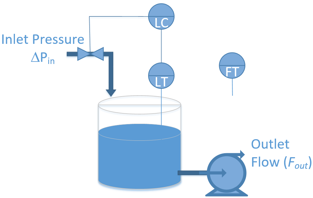
Note: The symbol LT is an abbreviation for Level Transmitter and FT for Flow Transmitter. The symbol LC is an abbreviation for Level Controller.
A beginning model is used below where the process equation is derived from a mass balance.
$$ \rho \; A \; \frac{dh}{dt} = \dot m_{in} - \dot m_{out} \quad \mathrm{with} \quad \dot m_{in} = \rho \; C_v \; lift \; \sqrt{\frac{\Delta P_{in}}{g_s}}$$
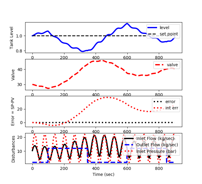
where `C_v=10^{-4}` relates valve opening and pressure drop `\Delta P_i` to inlet flow. The outlet water flow is a combination of pumped water rate and an unmeasured leak. Water has a specific gravity `g_s` of 1.0. Use a PI controller for the tank to maintain a level set point of 1.0 m. Test the PI controller with `K_c=20.0` and `tau_I=50.0` with feedforward and cascade control for a simulation period of 900 seconds (15 minutes). Use a value of 1000 kg/m3 for density and 5.0 m2 for the cross-sectional area of the tank. Assume a linear valve. Make sure that the valve does not exceed the limits of 0-100 percent by clipping the requested valve opening to an acceptable range. For example, if the PI controller calculates a valve opening of 150 percent, use 100 percent instead. Use the disturbance values for inlet pressure and outlet pressure included with the starting script to evaluate the effectiveness of the controller options. Create a plot of set point and level for each of the three cases.
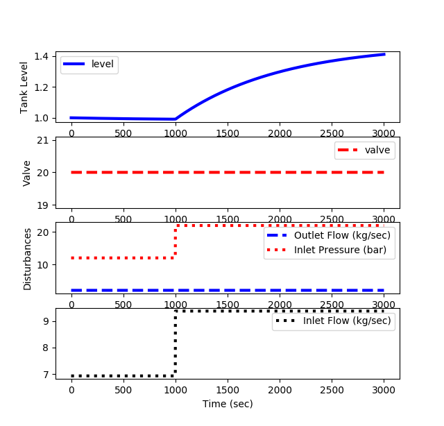
Step Response Simulation
import matplotlib.pyplot as plt
from scipy.integrate import odeint
import random
# define tank model
def tank(Level,time,valve,DeltaP,FlowOut):
Cv = 0.0001 # valve size
rho = 1000.0 # water density (kg/m^3)
A = 5.0 # tank area (m^2)
gs = 1.0 # specific gravity
# inlet mass flow
FlowIn = rho * Cv * valve * np.sqrt(DeltaP/gs)
# leak outlet flow
LeakOut = 5.0*Level
# calculate derivative of the Level
if Level <= 0.0:
dLevel_dt = 0.0 # for drained tank
else:
dLevel_dt = (FlowIn-FlowOut-LeakOut)/(rho*A)
return dLevel_dt
tf = 3000.0 # final time
n = int(tf + 1) # number of time points
# time span for the simulation, cycle every sec
ts = np.linspace(0,tf,n)
delta_t = ts[1] - ts[0]
# disturbances
DP = np.ones(n)*12.0
Fout = np.ones(n)*2.0
Fin = np.zeros(n)
# Desired level (set point)
SP = 1.0
# level initial condition
Level0 = SP
# initial valve position
valve = 20.0
# Controller bias
ubias = valve
# valve opening (0-100%)
u = np.ones(n) * valve
# for storing the results
z = np.ones(n)*Level0
Cv = 0.0001 # valve size
rho = 1000.0 # water density (kg/m^3)
A = 5.0 # tank area (m^2)
gs = 1.0 # specific gravity
################################################
# Step Response (uncomment select case)
# Case A
DP[1000:] = 22.0
# Case B
#u[1000:] = 30.0
# Case C
#Fout[1000:] = 3.0
################################################
# simulate with ODEINT
for i in range(n-1):
valve = u[i]
# inlet mass flow
Fin[i] = rho * Cv * valve * np.sqrt(DP[i]/gs)
#if i==500:
# valve = 30.0
#u[i+1] = valve # store the valve position
y = odeint(tank,Level0,[0,delta_t],args=(valve,DP[i],Fout[i]))
Level0 = y[-1] # take the last point
z[i+1] = Level0 # store the level for plotting
Fin[-1] = Fin[-2]
# plot results
plt.figure()
plt.subplot(4,1,1)
plt.plot(ts,z,'b-',linewidth=3,label='level')
plt.ylabel('Tank Level')
plt.legend(loc='best')
plt.subplot(4,1,2)
plt.plot(ts,u,'r--',linewidth=3,label='valve')
plt.ylabel('Valve')
plt.legend(loc=1)
plt.subplot(4,1,3)
plt.plot(ts,Fout,'b--',linewidth=3,label='Outlet Flow (kg/sec)')
plt.plot(ts,DP,'r:',linewidth=3,label='Inlet Pressure (bar)')
plt.ylabel('Disturbances')
plt.legend(loc=1)
plt.subplot(4,1,4)
plt.plot(ts,Fin,'k:',linewidth=3,label='Inlet Flow (kg/sec)')
plt.xlabel('Time (sec)')
plt.legend(loc=1)
plt.show()
PI Control Simulation
import matplotlib.pyplot as plt
from scipy.integrate import odeint
import random
# define tank model
def tank(Level,time,valve,DeltaP,FlowOut):
Cv = 0.0001 # valve size
rho = 1000.0 # water density (kg/m^3)
A = 5.0 # tank area (m^2)
gs = 1.0 # specific gravity
# inlet mass flow
FlowIn = rho * Cv * valve * np.sqrt(DeltaP/gs)
# leak outlet flow
LeakOut = 5.0*Level
# calculate derivative of the Level
if Level <= 0.0:
dLevel_dt = 0.0 # for drained tank
else:
dLevel_dt = (FlowIn-FlowOut-LeakOut)/(rho*A)
return dLevel_dt
tf = 900.0 # final time
n = int(tf + 1) # number of time points
# time span for the simulation, cycle every 1 sec
ts = np.linspace(0,tf,n)
delta_t = ts[1] - ts[0]
# disturbances
DP = np.zeros(n)
Fout = np.ones(n)*2.0
Fin = np.zeros(n)
# Desired level (set point)
SP = 1.0
# level initial condition
Level0 = SP
# initial valve position
valve = 30.0
# Controller bias
ubias = valve
# valve opening (0-100%)
u = np.ones(n) * valve
Cv = 0.0001 # valve size
rho = 1000.0 # water density (kg/m^3)
A = 5.0 # tank area (m^2)
gs = 1.0 # specific gravity
# for storing the results
z = np.ones(n)*Level0
es = np.zeros(n)
P = np.zeros(n) # proportional
I = np.zeros(n) # integral
ie = np.zeros(n)
# Controller tuning
Kc = 20.0
tauI = 50.0
# simulate with ODEINT
for i in range(n-1):
# inlet pressure (bar) disturbance
DP[i] = np.sin(ts[i]/10.0)* 10.0 + 12.0
# inlet mass flow
Fin[i] = rho * Cv * valve * np.sqrt(DP[i]/gs)
# outlet flow (kg/sec) disturbance (change every 10 seconds)
if np.mod(i+1,500)==100:
Fout[i] = Fout[i-1] + 10.0
elif np.mod(i+1,500)==350:
Fout[i] = Fout[i-1] - 10.0
else:
if i>=1:
Fout[i] = Fout[i-1]
# PI controller
# calculate the error
error = SP - Level0
P[i] = Kc * error
if i >= 1: # calculate starting on second cycle
ie[i] = ie[i-1] + error * delta_t
I[i] = (Kc/tauI) * ie[i]
valve = ubias + P[i] + I[i]
valve = max(0.0,valve) # lower bound = 0
valve = min(100.0,valve) # upper bound = 100
if valve > 100.0: # check upper limit
valve = 100.0
ie[i] = ie[i] - error * delta_t # anti-reset windup
if valve < 0.0: # check lower limit
valve = 0.0
ie[i] = ie[i] - error * delta_t # anti-reset windup
u[i+1] = valve # store the valve position
es[i+1] = error # store the error
y = odeint(tank,Level0,[0,delta_t],args=(valve,DP[i],Fout[i]))
Level0 = y[-1] # take the last point
z[i+1] = Level0 # store the level for plotting
Fout[n-1] = Fout[n-2]
DP[n-1] = DP[n-2]
Fin[n-1] = Fin[n-2]
ie[n-1] = ie[n-2]
# plot results
plt.figure()
plt.subplot(4,1,1)
plt.plot(ts,z,'b-',linewidth=3,label='level')
plt.plot([0,max(ts)],[SP,SP],'k--',linewidth=2,label='set point')
plt.ylabel('Tank Level')
plt.legend(loc=1)
plt.subplot(4,1,2)
plt.plot(ts,u,'r--',linewidth=3,label='valve')
plt.ylabel('Valve')
plt.legend(loc=1)
plt.subplot(4,1,3)
plt.plot(ts,es,'k:',linewidth=3,label='error')
plt.plot(ts,ie,'r:',linewidth=3,label='int err')
plt.legend(loc=1)
plt.ylabel('Error = SP-PV')
plt.subplot(4,1,4)
plt.plot(ts,Fin,'k-',linewidth=3,label='Inlet Flow (kg/sec)')
plt.plot(ts,Fout,'b--',linewidth=3,label='Outlet Flow (kg/sec)')
plt.plot(ts,DP,'r:',linewidth=3,label='Inlet Pressure (bar)')
plt.ylabel('Disturbances')
plt.xlabel('Time (sec)')
plt.legend(loc=1)
plt.show()
Solutions
# Controller tuning
Kff = -3.0
# simulate with ODEINT
for i in range(n-1):
##### add feedforward to controller
valve = ubias + P[i] + I[i] + Kff * (Fin[i]-Fin[0])
#####
import matplotlib.pyplot as plt
from scipy.integrate import odeint
import random
# define tank model
def tank(Level,time,valve,DeltaP,FlowOut):
Cv = 0.0001 # valve size
rho = 1000.0 # water density (kg/m^3)
A = 5.0 # tank area (m^2)
gs = 1.0 # specific gravity
# inlet mass flow
FlowIn = rho * Cv * valve * np.sqrt(DeltaP/gs)
# leak outlet flow
LeakOut = 5.0*Level
# calculate derivative of the Level
if Level <= 0.0:
dLevel_dt = 0.0 # for drained tank
else:
dLevel_dt = (FlowIn-FlowOut-LeakOut)/(rho*A)
return dLevel_dt
tf = 900.0 # final time
n = int(tf + 1) # number of time points
# time span for the simulation, cycle every 1 sec
ts = np.linspace(0,tf,n)
delta_t = ts[1] - ts[0]
# disturbances
DP = np.zeros(n)
Fout = np.ones(n)*2.0
Fin = np.zeros(n)
Fin_sp = np.zeros(n)
# Desired level (set point)
SP = 1.0
# level initial condition
Level0 = SP
# initial valve position
valve = 30.0
# Controller bias
ubias = valve
# valve opening (0-100%)
u = np.ones(n) * valve
Cv = 0.0001 # valve size
rho = 1000.0 # water density (kg/m^3)
A = 0.5 # tank area (m^2)
gs = 1.0 # specific gravity
# for storing the results
z = np.ones(n)*Level0
es = np.zeros(n)
P = np.zeros(n) # proportional
I = np.zeros(n) # integral
ie = np.zeros(n)
# Controller tuning
# Primary level controller
Kc_1 = 6.25
tauI_1 = 50.0
# Secondary flow controller
Kc_2 = 1.5
tauI_2 = 1.0
ierr2 = 0.0
# Feedforward control
Kff = 0.0 # 1.0
# simulate with ODEINT
for i in range(n-1):
# inlet pressure (bar) disturbance
DP[i] = np.sin(ts[i]/10.0)* 10.0 + 12.0
# inlet mass flow
Fin[i] = rho * Cv * valve * np.sqrt(DP[i]/gs)
# outlet flow (kg/sec) disturbance (change every 10 seconds)
if np.mod(i+1,500)==100:
Fout[i] = Fout[i-1] + 10.0
elif np.mod(i+1,500)==350:
Fout[i] = Fout[i-1] - 10.0
else:
if i>=1:
Fout[i] = Fout[i-1]
# PI controller (Primary Level Control)
# calculate the error
error = SP - Level0
P[i] = Kc_1 * error
if i >= 1: # calculate starting on second cycle
ie[i] = ie[i-1] + error * delta_t
I[i] = (Kc_1/tauI_1) * ie[i]
Fin_sp[i] = Fin[0] + P[i] + I[i] + Kff * (Fout[i]-Fout[0])
if Fin_sp[i] > 40.0: # check upper limit
Fin_sp[i] = 40.0
ie[i] = ie[i] - error * delta_t # anti-reset windup
if Fin_sp[i] < 0.0: # check lower limit
Fin_sp[i] = 0.0
ie[i] = ie[i] - error * delta_t # anti-reset windup
# PI controller (Secondary Flow Control)
# calculate the error
error2 = Fin_sp[i] - Fin[i]
P2 = Kc_2 * error2
ierr2 = ierr2 + error2 * delta_t
I2 = (Kc_2/tauI_2) * ierr2
valve = u[0] + P2 + I2
if valve > 100.0: # check upper limit
valve = 100.0
ierr2 = ierr2 - error2 * delta_t # anti-reset windup
if valve < 0.0: # check lower limit
valve = 0.0
ierr2 = ierr2 - error2 * delta_t # anti-reset windup
u[i+1] = valve # store the valve position
es[i+1] = error # store the error
y = odeint(tank,Level0,[0,delta_t],args=(valve,DP[i],Fout[i]))
Level0 = y[-1] # take the last point
z[i+1] = Level0 # store the level for plotting
Fout[n-1] = Fout[n-2]
DP[n-1] = DP[n-2]
Fin[n-1] = Fin[n-2]
Fin_sp[n-1] = Fin_sp[n-2]
ie[n-1] = ie[n-2]
# plot results
plt.figure()
plt.subplot(5,1,1)
plt.plot(ts,z,'b-',linewidth=3,label='level')
plt.plot([0,max(ts)],[SP,SP],'k--',linewidth=2,label='set point')
plt.ylabel('Tank Level')
plt.legend(loc=1)
plt.subplot(5,1,2)
plt.plot(ts,Fin_sp,'k-',linewidth=3,label='Inlet Flow SP')
plt.plot(ts,Fin,'r:',linewidth=3,label='Inlet Flow (kg/sec)')
plt.ylabel('Flow Control')
plt.legend(loc=1)
plt.subplot(5,1,3)
plt.plot(ts,u,'r--',linewidth=3,label='valve')
plt.ylabel('Valve')
plt.legend(loc=1)
plt.subplot(5,1,4)
plt.plot(ts,es,'k:',linewidth=3,label='error')
plt.plot(ts,ie,'r:',linewidth=3,label='int err')
plt.legend(loc=1)
plt.ylabel('Error = SP-PV')
plt.subplot(5,1,5)
plt.plot(ts,Fout,'b--',linewidth=3,label='Outlet Flow (kg/sec)')
plt.plot(ts,DP,'r:',linewidth=3,label='Inlet Pressure (bar)')
plt.ylabel('Disturbances')
plt.xlabel('Time (sec)')
plt.legend(loc=1)
plt.show()
# Controller tuning
Kff = 3.333
# simulate with ODEINT
for i in range(n-1):
##### add feedforward to controller
valve = ubias + P[i] + I[i] + Kff * (Fout[i]-Fout[0])
#####
What to Turn In
- Item 1: Brief description of controller architectures for Cases A–C (what you implemented and where the FT is installed).
- Item 2: Python code (or notebook) showing your PI level controller (Kc=20, `\tau_I`=50), valve clipping (0–100%), and the feedforward/cascade additions for each case.
- Item 3: Three plots (one per case) of level vs. time with setpoint over 900 s, plus any auxiliary traces you used (valve %, inlet/outlet flow, inlet pressure).
- Item 4: Quantitative performance summary for each case (e.g., max |SP–PV|, settling time, overshoot, IAE/ISE or your chosen metric).
- Item 5: Comparison and discussion: which FT placement (inlet vs. outlet) and which strategy (feedforward vs. cascade) best rejects `ΔP`in and `ṁ_{out}` disturbances, and why (tie your rationale to the model/assumptions such as `θ_p` vs. `θ_d` and inner-loop bandwidth requirements).
- Item 6: Final recommendation for transmitter placement and control configuration (A, B, or C) for this tank with brief justification.