Distillate Composition Control
 |  |  |  |
|---|
Over 40,000 distillation columns in the U.S. consume 40-60% of the total energy in the petrochemical industry and 6% of the total U.S. energy usage. Reducing distillation energy usage would have a major impact on energy independence, greenhouse gas emissions, and give a competitive advantage to any manufacturer that is better able to implement improvements.
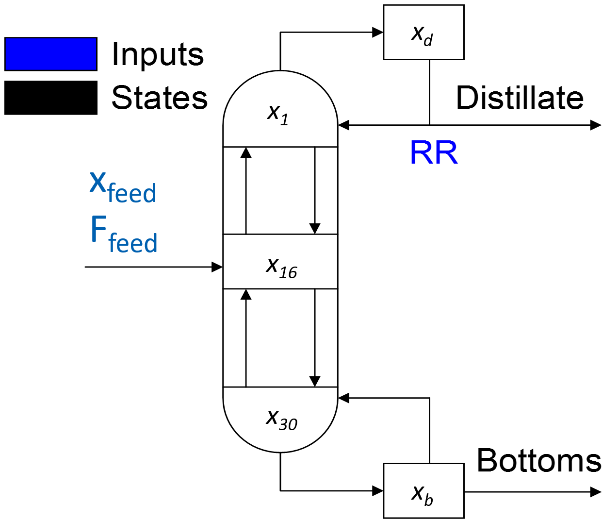
The objective of this exercise is to maintain an overhead mole fraction for the light component in a binary distillation column that separates cyclohexane and n-heptane. The nominal steady state for the column is a reflux ratio at 3.0 with an allowable range from 1.0 to 10.0. This reflux ratio produces a cyclohexane product with a purity of 0.935 (mole fraction), but the target composition is 0.970 with an allowable range of 0.960 to 0.980. The objective is to design a PID controller to meet this target value and stay within the specified product range.
Manipulated Variable: Reflux Ratio: RR (Ratio of distillate flowrate returning to the column divided by the flowrate of the product leaving)
Controlled Variable: Distillate composition `(x_d)` mole fraction
Measured Disturbances: (1) Feed flow rate, (2) Feed composition (mole fraction)
Determine Steady State Conditions
Report the design set point and controller bias `u_{bias}` value for the controller.
Estimate Model
Perform a doublet test and use the dynamic response data to estimate a first order plus dead time (FOPDT) model.
import matplotlib.pyplot as plt
from scipy.integrate import odeint
# define model
def distill(x,t,rr,Feed,x_Feed):
# Inputs (3):
# Reflux ratio is the Manipulated variable
# Reflux Ratio (L/D)
#rr = p(1)
# Disturbance variables (DV)
# Feed Flowrate (mol/min)
#Feed = p(2)
# Mole Fraction of Feed
#x_Feed = p(3)
# States (32):
# x(0) - Reflux Drum Liquid Mole Fraction of Component A
# x(1) - Tray 1 - Liquid Mole Fraction of Component A
# .
# .
# .
# x(16) - Tray 16 - Liquid Mole Fraction of Component A (Feed)
# .
# .
# .
# x(30) - Tray 30 - Liquid Mole Fraction of Component A
# x(31) - Reboiler Liquid Mole Fraction of Component A
# Parameters
# Distillate Flowrate (mol/min)
D=0.5*Feed
# Flowrate of the Liquid in the Rectification Section (mol/min)
L=rr*D
# Vapor Flowrate in the Column (mol/min)
V=L+D
# Flowrate of the Liquid in the Stripping Section (mol/min)
FL=Feed+L
# Relative Volatility = (yA/xA)/(yB/xB) = KA/KB = alpha(A,B)
vol=1.6
# Total Molar Holdup in the Condenser
atray=0.25
# Total Molar Holdup on each Tray
acond=0.5
# Total Molar Holdup in the Reboiler
areb=1.0
# Vapor Mole Fractions of Component A
# From the equilibrium assumption and mole balances
# 1) vol = (yA/xA) / (yB/xB)
# 2) xA + xB = 1
# 3) yA + yB = 1
y = np.empty(len(x))
for i in range(32):
y[i] = x[i] * vol/(1.0+(vol-1.0)*x[i])
# Compute xdot
xdot = np.empty(len(x))
xdot[0] = 1/acond*V*(y[1]-x[0])
for i in range(1,16):
xdot[i] = 1.0/atray*(L*(x[i-1]-x[i])-V*(y[i]-y[i+1]))
xdot[16] = 1/atray*(Feed*x_Feed+L*x[15]-FL*x[16]-V*(y[16]-y[17]))
for i in range(17,31):
xdot[i] = 1.0/atray*(FL*(x[i-1]-x[i])-V*(y[i]-y[i+1]))
xdot[31] = 1/areb*(FL*x[30]-(Feed-D)*x[31]-V*y[31])
return xdot
# Steady State Initial Conditions for the 32 states
x_ss =np.array([0.935,0.900,0.862,0.821,0.779,0.738,\
0.698,0.661,0.628,0.599,0.574,0.553,0.535,0.521, \
0.510,0.501,0.494,0.485,0.474,0.459,0.441,0.419, \
0.392,0.360,0.324,0.284,0.243,0.201,0.161,0.125, \
0.092,0.064])
x0 = x_ss
# Steady State Initial Condition
rr_ss = 3.0
# Time Interval (min)
t = np.linspace(0,50,500)
# Store results for plotting
xd = np.ones(len(t)) * x_ss[0]
rr = np.ones(len(t)) * rr_ss
ff = np.ones(len(t))
xf = np.ones(len(t)) * 0.5
sp = np.ones(len(t)) * 0.935
# Step in reflux ratio
rr[10:] = 1.0
rr[180:] = 5.0
rr[360:] = 3.0
plt.figure(figsize=(10,7))
plt.ion()
plt.show()
# Simulate
for i in range(len(t)-1):
ts = [t[i],t[i+1]]
y = odeint(distill,x0,ts,args=(rr[i],ff[i],xf[i]))
xd[i+1] = y[-1][0]
x0 = y[-1]
# Plot the results
plt.clf()
plt.subplot(2,1,1)
plt.plot(t[0:i+1],rr[0:i+1],'b--',linewidth=3)
plt.ylabel(r'$RR$')
plt.legend(['Reflux ratio'],loc='best')
plt.subplot(2,1,2)
plt.plot(t[0:i+1],sp[0:i+1],'k.-',linewidth=1)
plt.plot(t[0:i+1],xd[0:i+1],'r-',linewidth=3)
plt.ylabel(r'$x_d\;(mol/L)$')
plt.legend(['Starting composition','Distillate composition'],loc='best')
plt.xlabel('Time (hr)')
plt.draw()
plt.pause(0.05)
# Construct results and save data file
# Column 1 = time
# Column 2 = reflux ratio
# Column 3 = distillate composition
data = np.vstack((t,rr,xd)) # vertical stack
data = data.T # transpose data
np.savetxt('data.txt',data,delimiter=',')
plt.savefig('distillation.png')
Obtain PID Parameters
Use the FOPDT model values in the IMC tuning correlation to compute the tuning constants `K_c`, `\tau_I`, and `\tau_D`. Specify the sign, magnitude, and units of each.
Implement PID Controller
Using the design set point, bias, and controller gain, implement the PID controller. Generate a plot showing the performance of the controller in tracking the set point.
Set Point Changes
Fine tune the controller gain by trial and error and search for the best parameters that balance speed with oscillatory behavior when tracking this set point from 0.935 to 0.970. Remember that as the designer, define what constitutes best performance. As well as generating a plot with final tuning, explain what criteria you is used to define best.
Disturbance Rejection
Introduce a disturbance in the feed after 50 minutes by changing the mole fraction from 0.50 to 0.42. Tune the controller to stay within the desired product range given this disturbance. If the controller isn't able to keep within the desirable range, discuss if it is possible to improve the control.
Distillation Simulation Code
Use the open loop simulation code as a starting point for the problem. There are 30 trays, 1 reboiler, and 1 condenser for this simulation. The 32 states are updated with every cycle of the simulation loop but only the distillate composition is measured.
import matplotlib.pyplot as plt
from scipy.integrate import odeint
# define model
def distill(x,t,rr,Feed,x_Feed):
# Inputs (3):
# Reflux ratio is the Manipulated variable
# Reflux Ratio (L/D)
#rr = p(1)
# Disturbance variables (DV)
# Feed Flowrate (mol/min)
#Feed = p(2)
# Mole Fraction of Feed
#x_Feed = p(3)
# States (32):
# x(0) - Reflux Drum Liquid Mole Fraction of Component A
# x(1) - Tray 1 - Liquid Mole Fraction of Component A
# .
# .
# .
# x(16) - Tray 16 - Liquid Mole Fraction of Component A (Feed)
# .
# .
# .
# x(30) - Tray 30 - Liquid Mole Fraction of Component A
# x(31) - Reboiler Liquid Mole Fraction of Component A
# Parameters
# Distillate Flowrate (mol/min)
D=0.5*Feed
# Flowrate of the Liquid in the Rectification Section (mol/min)
L=rr*D
# Vapor Flowrate in the Column (mol/min)
V=L+D
# Flowrate of the Liquid in the Stripping Section (mol/min)
FL=Feed+L
# Relative Volatility = (yA/xA)/(yB/xB) = KA/KB = alpha(A,B)
vol=1.6
# Total Molar Holdup in the Condenser
atray=0.25
# Total Molar Holdup on each Tray
acond=0.5
# Total Molar Holdup in the Reboiler
areb=1.0
# Vapor Mole Fractions of Component A
# From the equilibrium assumption and mole balances
# 1) vol = (yA/xA) / (yB/xB)
# 2) xA + xB = 1
# 3) yA + yB = 1
y = np.empty(len(x))
for i in range(32):
y[i] = x[i] * vol/(1.0+(vol-1.0)*x[i])
# Compute xdot
xdot = np.empty(len(x))
xdot[0] = 1/acond*V*(y[1]-x[0])
for i in range(1,16):
xdot[i] = 1.0/atray*(L*(x[i-1]-x[i])-V*(y[i]-y[i+1]))
xdot[16] = 1/atray*(Feed*x_Feed+L*x[15]-FL*x[16]-V*(y[16]-y[17]))
for i in range(17,31):
xdot[i] = 1.0/atray*(FL*(x[i-1]-x[i])-V*(y[i]-y[i+1]))
xdot[31] = 1/areb*(FL*x[30]-(Feed-D)*x[31]-V*y[31])
return xdot
# Steady State Initial Conditions for the 32 states
x_ss =np.array([0.935,0.900,0.862,0.821,0.779,0.738,\
0.698,0.661,0.628,0.599,0.574,0.553,0.535,0.521, \
0.510,0.501,0.494,0.485,0.474,0.459,0.441,0.419, \
0.392,0.360,0.324,0.284,0.243,0.201,0.161,0.125, \
0.092,0.064])
x0 = x_ss
# Steady State Initial Condition
rr_ss = 3.0
# Time Interval (min)
t = np.linspace(0,10,100)
# Store results for plotting
xd = np.ones(len(t)) * x_ss[0]
rr = np.ones(len(t)) * rr_ss
ff = np.ones(len(t))
xf = np.ones(len(t)) * 0.5
sp = np.ones(len(t)) * 0.97
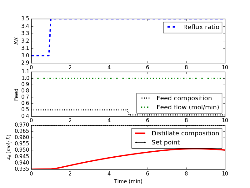
# Step in reflux ratio
rr[10:] = 3.5
# Feed Concentration (mol frac)
xf[50:] = 0.42
# Feed flow rate
ff[80:] = 1.0
plt.figure(figsize=(10,7))
plt.ion()
plt.show()
# Simulate
for i in range(len(t)-1):
ts = [t[i],t[i+1]]
y = odeint(distill,x0,ts,args=(rr[i],ff[i],xf[i]))
xd[i+1] = y[-1][0]
x0 = y[-1]
# Plot the results
plt.clf()
plt.subplot(3,1,1)
plt.plot(t[0:i+1],rr[0:i+1],'b--',linewidth=3)
plt.ylabel(r'$RR$')
plt.legend(['Reflux ratio'],loc='best')
plt.subplot(3,1,2)
plt.plot(t[0:i+1],xf[0:i+1],'k:',linewidth=3,label='Feed composition')
plt.plot(t[0:i+1],ff[0:i+1],'g-.',linewidth=3,label='Feed flow (mol/min)')
plt.ylabel('Feed')
plt.ylim([0.4,1.1])
plt.legend(loc='best')
plt.subplot(3,1,3)
plt.plot(t[0:i+1],xd[0:i+1],'r-',linewidth=3)
plt.plot(t[0:i+1],sp[0:i+1],'k.-',linewidth=1)
plt.ylabel(r'$x_d\;(mol/L)$')
plt.legend(['Distillate composition','Set point'],loc='best')
plt.xlabel('Time (min)')
plt.draw()
plt.pause(0.05)
# Construct results and save data file
# Column 1 = time
# Column 2 = reflux ratio
# Column 3 = distillate composition
data = np.vstack((t,rr,xd)) # vertical stack
data = data.T # transpose data
np.savetxt('data.txt',data,delimiter=',')
plt.savefig('distillation.png')
Solutions
Solutions videos are available in Python (see below) and MATLAB.
import matplotlib.pyplot as plt
from scipy.integrate import odeint
# define model
def distill(x,t,rr,Feed,x_Feed):
# Inputs (3):
# Reflux ratio is the Manipulated variable
# Reflux Ratio (L/D)
#rr = p(1)
# Disturbance variables (DV)
# Feed Flowrate (mol/min)
#Feed = p(2)
# Mole Fraction of Feed
#x_Feed = p(3)
# States (32):
# x(0) - Reflux Drum Liquid Mole Fraction of Component A
# x(1) - Tray 1 - Liquid Mole Fraction of Component A
# .
# .
# .
# x(16) - Tray 16 - Liquid Mole Fraction of Component A (Feed)
# .
# .
# .
# x(30) - Tray 30 - Liquid Mole Fraction of Component A
# x(31) - Reboiler Liquid Mole Fraction of Component A
# Parameters
# Distillate Flowrate (mol/min)
D=0.5*Feed
# Flowrate of the Liquid in the Rectification Section (mol/min)
L=rr*D
# Vapor Flowrate in the Column (mol/min)
V=L+D
# Flowrate of the Liquid in the Stripping Section (mol/min)
FL=Feed+L
# Relative Volatility = (yA/xA)/(yB/xB) = KA/KB = alpha(A,B)
vol=1.6
# Total Molar Holdup in the Condenser
atray=0.25
# Total Molar Holdup on each Tray
acond=0.5
# Total Molar Holdup in the Reboiler
areb=1.0
# Vapor Mole Fractions of Component A
# From the equilibrium assumption and mole balances
# 1) vol = (yA/xA) / (yB/xB)
# 2) xA + xB = 1
# 3) yA + yB = 1
y = np.empty(len(x))
for i in range(32):
y[i] = x[i] * vol/(1.0+(vol-1.0)*x[i])
# Compute xdot
xdot = np.empty(len(x))
xdot[0] = 1/acond*V*(y[1]-x[0])
for i in range(1,16):
xdot[i] = 1.0/atray*(L*(x[i-1]-x[i])-V*(y[i]-y[i+1]))
xdot[16] = 1/atray*(Feed*x_Feed+L*x[15]-FL*x[16]-V*(y[16]-y[17]))
for i in range(17,31):
xdot[i] = 1.0/atray*(FL*(x[i-1]-x[i])-V*(y[i]-y[i+1]))
xdot[31] = 1/areb*(FL*x[30]-(Feed-D)*x[31]-V*y[31])
return xdot
# Steady State Initial Conditions for the 32 states
x_ss =np.array([0.935,0.900,0.862,0.821,0.779,0.738,\
0.698,0.661,0.628,0.599,0.574,0.553,0.535,0.521, \
0.510,0.501,0.494,0.485,0.474,0.459,0.441,0.419, \
0.392,0.360,0.324,0.284,0.243,0.201,0.161,0.125, \
0.092,0.064])
x0 = x_ss
# Steady State Initial Condition
rr_ss = 3.0
# Time Interval (min)
ns = 101
t = np.linspace(0,100,ns)
# Store results for plotting
xd = np.ones(len(t)) * x_ss[0]
rr = np.ones(len(t)) * rr_ss
ff = np.ones(len(t))
xf = np.ones(len(t)) * 0.5
# Step in reflux ratio
#rr[10:] = 4.0
#rr[40:] = 2.0
#rr[70:] = 3.0
# Feed Concentration (mol frac)
xf[50:] = 0.42
# Feed flow rate
#ff[80:] = 1.0
delta_t = t[1]-t[0]
# storage for recording values
op = np.ones(ns)*3.0 # controller output
pv = np.zeros(ns) # process variable
e = np.zeros(ns) # error
ie = np.zeros(ns) # integral of the error
dpv = np.zeros(ns) # derivative of the pv
P = np.zeros(ns) # proportional
I = np.zeros(ns) # integral
D = np.zeros(ns) # derivative
sp = np.ones(ns)*0.935 # set point
sp[10:] = 0.97
# PID (tuning)
Kc = 60
tauI = 4
tauD = 0.0
# Upper and Lower limits on OP
op_hi = 10.0
op_lo = 1.0
# loop through time steps
for i in range(1,ns):
e[i] = sp[i] - pv[i]
if i >= 1: # calculate starting on second cycle
dpv[i] = (pv[i]-pv[i-1])/delta_t
ie[i] = ie[i-1] + e[i] * delta_t
P[i] = Kc * e[i]
I[i] = Kc/tauI * ie[i]
D[i] = - Kc * tauD * dpv[i]
op[i] = op[0] + P[i] + I[i] + D[i]
if op[i] > op_hi: # check upper limit
op[i] = op_hi
ie[i] = ie[i] - e[i] * delta_t # anti-reset windup
if op[i] < op_lo: # check lower limit
op[i] = op_lo
ie[i] = ie[i] - e[i] * delta_t # anti-reset windup
# distillation solution (1 time step)
rr[i] = op[i]
ts = [t[i-1],t[i]]
y = odeint(distill,x0,ts,args=(rr[i],ff[i],xf[i]))
xd[i] = y[-1][0]
x0 = y[-1]
if i<ns-1:
pv[i+1] = y[-1][0]
#op[ns] = op[ns-1]
#ie[ns] = ie[ns-1]
#P[ns] = P[ns-1]
#I[ns] = I[ns-1]
#D[ns] = D[ns-1]
# Construct results and save data file
# Column 1 = time
# Column 2 = reflux ratio
# Column 3 = distillate composition
data = np.vstack((t,rr,xd)) # vertical stack
data = data.T # transpose data
np.savetxt('data.txt',data,delimiter=',')
# Plot the results
plt.figure()
plt.subplot(3,1,1)
plt.plot(t,rr,'b--',linewidth=3)
plt.ylabel(r'$RR$')
plt.legend(['Reflux ratio'],loc='best')
plt.subplot(3,1,2)
plt.plot(t,xf,'k:',linewidth=3,label='Feed composition')
plt.plot(t,ff,'g-.',linewidth=3,label='Feed flow (mol/min)')
plt.ylabel('Feed')
plt.ylim([0.4,1.1])
plt.legend(loc='best')
plt.subplot(3,1,3)
plt.plot(t,xd,'r-',linewidth=3)
plt.plot(t,sp,'k.-',linewidth=1)
plt.ylabel(r'$x_d\;(mol/L)$')
plt.legend(['Distillate composition','Set point'],loc='best')
plt.xlabel('Time (min)')
plt.savefig('distillation.png')
plt.show()