Nonlinear Pricing
Companies determine a demand curve by analyzing the relationship between the price of a product or service and the quantity that customers are willing to purchase at different prices. Here are a few methods that companies use to estimate the demand curve:
1️⃣ Surveys: Companies can conduct surveys to understand how much customers are willing to pay for their product or service. They can ask customers how much they would be willing to pay at different price points and use this data to estimate the demand curve.
2️⃣ Historical Sales Data: Companies analyze historical sales data to understand how changes in price have affected the quantity sold. By plotting the sales data against the different prices, they estimate the demand curve.
3️⃣ Experiments: Companies conduct experiments to test the demand for their product or service at different prices. They can offer discounts or run promotions to understand how customers respond to different price points.
4️⃣ Market Research: Companies conduct market research to understand the broader market and competition. By understanding how customers view their product or service in relation to other options in the market, they can estimate the demand curve.
Once a company has estimated the demand curve, they use this information to set prices that maximize profit. Sometimes they charge the same price for everyone. Other times they charge different prices to different customers based on their willingness to pay.
Nonlinear Pricing Example
A nonlinear pricing model is provided as an example in Practical Management Science by Wayne L. Winston and S. Christian Albright. Instead of solving the problem with a spreadsheet, the optimization and visualization of the optimal pricing is performed with Python.
Demand
The demand (d) decreases with increasing price (p) according to the constant elasticity demand curve:
$$d = 3777178 \, p^{-2.154}$$
Total Profit
It costs $50 to produce the item. The total profit is the product of the demand and individual profit per unit sold. The objective is to maximize the total profit.
$$\max \, (p-50) \, d$$
Python Solution
The following is a solution with Python using the Gekko package (pip install gekko) to find the optimal price for a product that maximizes profit, given the demand curve.
m = GEKKO()
p = m.Var(lb=50) # price
d = m.Var(lb=100) # demand
m.Equation(d == 3.777178e6*p**(-2.154))
m.Maximize((p-50)*d)
m.solve()
print('Solution')
price = p.value[0]
obj = -m.options.objfcnval
print(f'Price: ${price:0.2f}')
print(f'Profit: ${obj:0.2f}')
The code first creates a GEKKO model object m. It then creates two variables p and d, which represent the price and demand for the product, respectively. The lb parameter sets the lower bound for the variables. Next, the code sets an equation that models the demand curve using the Equation method. The demand curve in this example is a power function of the form `d = a p^(-b)`, where a and b are constants. The code then uses the Maximize method to set the objective function, which is the profit equation (p - 50) * d. This represents the revenue from selling the product at price p minus the fixed costs of producing the product. The solve method is called to solve the optimization problem and find the optimal price that maximizes profit. The optimal price and profit are then printed to the console.
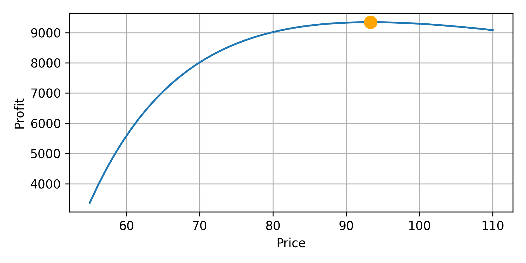
  Solution
  Price: $93.33
  Profit: $9343.95
View Optimal Solution and Profit Curve
Numpy and Matplotlib are used to view the optimal solution and the nonlinear relationship between price and total profit. The total profit curve shows that the price can vary between $80 and $112 and still remain above $9000 total profit.
import matplotlib.pyplot as plt
px = np.linspace(55,110)
dx = 3.777178e6*px**(-2.154)
profit = (px-50)*dx
plt.figure(figsize=(6,3))
plt.plot(px,profit)
plt.plot(price,obj,'o',markersize=10,color='orange')
plt.grid(); plt.xlabel('Price'); plt.ylabel('Profit')
plt.tight_layout()
plt.show()
It may be desirable to reduce total profit for competitive reasons or to keep the supply chain full. A possible strategy is to set the price at $80 to keep competitors out of the market. Another possible strategy is to raise the price to $112 if there are logistic concerns with suppliers so that production is lowered.
Demand Curve Uncertainty
Deciding on a price point can be challenging when there is demand uncertainty. In addition to understanding the market and testing the pricing, there are additional factors that can give guidance on the pricing strategy:
- Analyze the costs: Determine fixed and variable costs and calculate a break-even point. This determines the minimum price to charge to cover costs.
- Consider value: Determine the unique value proposition of the product or service and how much customers are willing to pay for it. This can help you set a premium price point.
- Monitor demand: Keep an eye on demand trends and adjust pricing strategy accordingly. If demand is higher than expected, consider raising the price to avoid supply shortages.
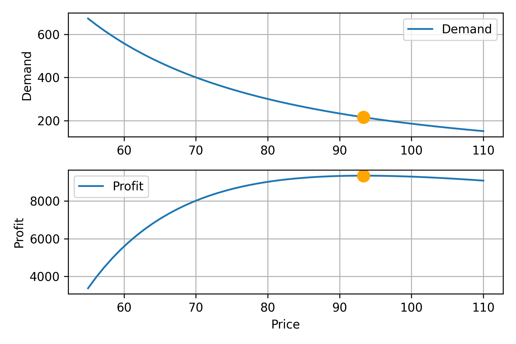
px = np.linspace(55,110)
dx = 3.777178e6*px**(-2.154)
profit = (px-50)*dx
import matplotlib.pyplot as plt
plt.figure(figsize=(6,4))
plt.subplot(2,1,1)
plt.plot(px,dx,label='Demand')
plt.plot(price,d.value[0],'o',markersize=10,color='orange')
plt.grid(); plt.ylabel('Demand'); plt.legend()
plt.subplot(2,1,2)
plt.plot(px,profit,label='Profit')
plt.plot(price,obj,'o',markersize=10,color='orange')
plt.grid(); plt.legend()
plt.xlabel('Price'); plt.ylabel('Profit')
plt.tight_layout(); plt.savefig('results.png',dpi=300)
plt.show()
A feedback control mechanism can be used to ensure product or service availability. This strategy is a dynamic price point that raises or lowers the price as the supply fluctuates. Optimization strategies can also include uncertainty that is quantified with regression statistics, Gaussian Processes, and other regression methods.