Estimate Thermodynamic Parameters from Data
Thermodynamic Parameter Estimation
Using data from an ebulliometer, determine parameters for a Vapor Liquid Equilibrium chart using the Wilson activity coefficient model with measured data for an ethanol-cyclohexane mixture at ambient pressure. Use the results to determine whether there is:
- An azeotrope in the system and, if so, at what composition
- The values of the activity coefficients at the infinitely dilute compositions
- gamma1 at x1=0
- gamma2 at x1=1
The liquid and vapor compositions of this binary mixture are related by the following thermodynamic relationships
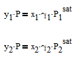
where y1is the vapor mole fraction, P is the pressure, x1 is the liquid mole fraction, gamma1 is the activity coefficient that is different than 1.0 for non-ideal mixtures, and P1sat is the pure component vapor pressure. The same equation also applies to component 2 in the mixture with the corresponding equation with subscript 2.
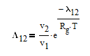
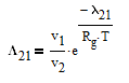
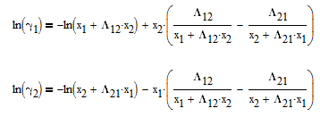
The Wilson equation is used to predict the activity coefficients gamma2 and gamma2 over the range of liquid compositions.
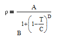
There are correlations for Psat1 and density (rho) for many common pure components from BYU's DIPPR database. In this case P1sat is a function of temperature according to
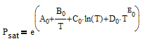
and density rho or molar volume v is also a function of temperature according to

The number of degrees of freedom in a multi-component and multi-phase system is given by DOF = 2 + #Components - #Phases. In this case, there are two phases (liquid and vapor) and two components (ethanol and cyclohexane). This leads to two degrees of freedom that must be specified. In this case, we can chose to fix two of the four measured values for this system with either x1, y1, P, or T. It is recommended to fix the values of x1 and P as shown in the tutorial below.
APM Python

Python GEKKO
import numpy as np
import pandas as pd
import matplotlib.pyplot as plt
from scipy.optimize import fsolve
from scipy.optimize import curve_fit
from scipy.interpolate import interp1d
#from numpy import *
R = 1.9858775 # cal/mol K
def vaporP(T: float, component: list):
'''
:param T: temp [K]
:param component: [vapor pressure parameters]
:return: Vapor Pressure [Pa]
'''
A = component[0]
B = component[1]
C = component[2]
D = component[3]
E = component[4]
return np.exp(A + B/T + C*np.log(T) + D*T**E)
def liquidMolarVolume(T: float, component: list):
'''
:param T: temp in [K}
:param component: component liquid molar volume
: constants in list or array
:return: liquid molar volume []
'''
A = component[0]
B = component[1]
C = component[2]
D = component[3]
return 1 / A * B ** (1 + (1 - T / C) ** D)
def Lij(aij: float, T: float, Vlvali: float,\
Vlvalj: float):
# Vl1 = liquidMolarVolume(T, Vlvali)
# Vl2 = liquidMolarVolume(T, Vlvalj)
Vl1 = Vlvali
Vl2 = Vlvalj
return Vl2 / Vl1 * np.exp(-aij / (R * T))
def Gamma(a12: float, a21: float, x1: float,\
Temp: float, Component: int):
'''
:param Component:
:param a12:
:param a21:
:param x1:
:param Temp:
:return:
'''
# Liquid molar volume
Vethanol = 5.8492e-2
VCyclochexane = 0.10882
x2 = 1.0 - x1
L12 = Lij(a12, Temp, Vethanol, VCyclochexane)
L21 = Lij(a21, Temp, VCyclochexane, Vethanol)
L11 = 1.0
L22 = 1.0
if Component == 1:
A = x1 + x2 * L12
B = x1 * L11 / (x1 * L11 + x2 * L12) \
+x2 * L21 / (x1 * L21 + x2 * L22)
elif Component == 2:
A = x2 + x1 * L21
B = x2 * L22 / (x2 * L22 + x1 * L21) \
+x1 * L12 / (x2 * L12 + x1 * L11)
return np.exp(1.0 - np.log(A) - B)
# yi * P = xi * γi * Pisat
# Component 1: Ethanol
# Component 2: Cyclohexane
def massTOMoleF(x: list):
#Converts RI to mole fraction of Ethanol
MW_Ethanol = 46.06844
MW_cyclohexane = 84.15948
xeth = 49.261*x**2 - 152.51*x + 117.32
xcyc = 1-xeth
moleth = xeth / MW_Ethanol
molcyc = xcyc/ MW_cyclohexane
return moleth/ (moleth + molcyc)
#Read in actual data
#filename = 'RealData.csv'
filename = 'http://apmonitor.com/me575/uploads/Main/vle_data.txt'
data = pd.read_csv(filename)
temp_data = data['Temp_D'].values + 273.15 # K
IndexMeasuredY = data['Distills_RI']
IndexMeasuredX = data['Bottoms_RI']
x1_data = massTOMoleF(IndexMeasuredX)
x1_data[0] = 0
x1_data[1] = 1
y1_data = massTOMoleF(IndexMeasuredY)
y1_data[0] = 0
y1_data[1] = 1
# Ethanol & Cyclohexane Properties ---------
# Psat paramater values
PsatC2H5OH = [73.304, -7122.3, -7.1424, \
2.8853e-6, 2.0]
PsatC6H12 = [51.087, -5226.4, -4.2278, \
9.7554e-18, 6.0]
# thermo Liquid Molar Volume paramaters
Vl_C2H5OH = [1.6288, 0.27469, 514.0, 0.23178]
Vl_C6H12 = [0.88998, 0.27376, 553.8, 0.28571]
# Build Model ------------------------------
m = GEKKO()
# Define Variables & Parameters
a12_ = m.FV(value = 2026.3)
a12_.STATUS = 1
a21_ = m.FV(value = 390.4)
a21_.STATUS = 1
Temp = m.Var(333)
x1 = m.Param(value = np.array(x1_data))
y1 = m.CV(value = np.array(y1_data))
y1.FSTATUS = 1 # min fstatus * (meas-pred)^2
y2 = m.Intermediate(1.0 - y1)
P = 85900 # Pa in Provo, UT
# Calc Vapor pressures of ethanol & cyclohexane at
# different temps using thermo parameters
# Psat = exp(A + B / T + C * log(T) + D * T ** E)
PsatEthanol = m.Intermediate(
m.exp(
PsatC2H5OH[0] +
PsatC2H5OH[1] / Temp +
PsatC2H5OH[2] * m.log(Temp) +
PsatC2H5OH[3] * Temp ** PsatC2H5OH[4]
)
)
PsatCyclohexane = m.Intermediate(
m.exp(
PsatC6H12[0] +
PsatC6H12[1] / Temp +
PsatC6H12[2] * m.log(Temp) +
PsatC6H12[3] * Temp ** PsatC6H12[4]
)
)
# Calculate Liquid Molar volumes of components 1 and 2:
# ethanol & cyclohexane, respectively
LMV_C2H5OH = 5.8492e-2
LMV_C6H12 = 0.10882
# Construct parameters for Wilson Model
L12 = m.Intermediate(LMV_C6H12 / LMV_C2H5OH \
* m.exp(-a12_ / (R * Temp)))
L21 = m.Intermediate(LMV_C2H5OH / LMV_C6H12 \
* m.exp(-a21_ / (R * Temp)))
L11 = 1.0
L22 = 1.0
x2 = m.Intermediate(1.0 - x1)
A1 = m.Intermediate(x1 + x2 * L12)
B1 = m.Intermediate(x1 * L11 / (x1 * L11 + x2 * L12) \
+ x2 * L21 / (x1 * L21 + x2 * L22))
A2 = m.Intermediate(x2 + x1 * L21)
B2 = m.Intermediate(x2 * L22 / (x2 * L22 + x1 * L21) \
+ x1 * L12 / (x2 * L12 + x1 * L11))
# Find Gammas for each component
G_C2H5OH = m.Intermediate(m.exp(1.0 - m.log(A1) - B1))
G_C6H12 = m.Intermediate(m.exp(1.0 - m.log(A2) - B2))
m.Equation(y2 == (G_C6H12 * PsatCyclohexane / P) * x2)
m.Equation(y1 == (G_C2H5OH * PsatEthanol / P) * x1)
# Options
m.options.IMODE = 2
m.options.EV_TYPE = 2 # Objective type, SSE
m.options.NODES = 3 # Collocation nodes
m.options.SOLVER = 3 # IPOPT
m.solve()
regressed_a12 = a12_.value[-1]
regressed_a21 = a21_.value[-1]
a12_Hysys = 2026.3
a21_Hysys = 390.4
x1_linspace = np.linspace(0, 1.0, 100)
y1_predicted = []
T_predicted = []
print("Activity Coefficient Parameters")
print('Model a12 a21')
print('Gekko: ' + str(round(regressed_a12,2)) \
+ str(round(regressed_a21,2)))
print('Hysys: ' + str(round(a12_Hysys,2)) \
+ str(round(a21_Hysys,2)))
def getValues(y1_and_Temp: list, a12: float, \
a21: float, P: float, x1: float):
y1 = y1_and_Temp[0]
T = y1_and_Temp[1]
y2 = 1 - y1
x2 = 1 - x1
A = y1*P - x1*Gamma(a12,a21,x1,T,1) \
* vaporP(T,PsatC2H5OH)
B = y2*P - x2*Gamma(a12,a21,x1,T,2) \
* vaporP(T,PsatC6H12)
return [A,B]
TempInterp = interp1d(x1_data, temp_data)
for i in range(len(x1_linspace)):
answers = fsolve(getValues, [x1_linspace[i],\
TempInterp(x1_linspace[i])],\
args = (regressed_a12, \
regressed_a21, \
P, x1_linspace[i]))
y1_predicted.append(answers[0])
T_predicted.append(answers[1])
GammaPred = Gamma(regressed_a12, regressed_a21, \
x1_data, temp_data, 1)
GammaPredHysys = Gamma(a12_Hysys, a21_Hysys, \
x1_data, temp_data, 2)
VP_Ethanol = vaporP(temp_data, PsatC2H5OH)
y1Predicted = (GammaPred * VP_Ethanol / P) * x1_data
y1PredictedHysys = (GammaPredHysys * VP_Ethanol / P) * x1_data
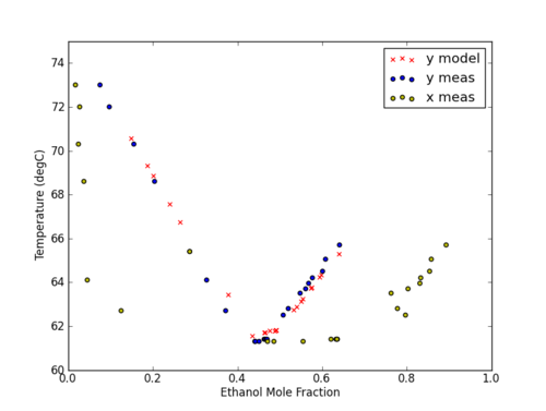
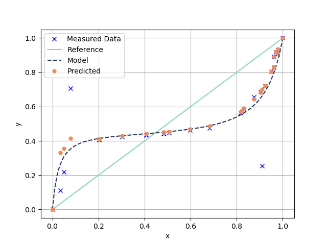
plt.figure(1)
plt.plot(x1_data,y1_data,"bx",label = "Measured Data")
plt.plot(x1_linspace,x1_linspace,"-",\
color="#8bd8bd", label="Reference",markersize=7)
plt.plot(x1_linspace,y1_predicted,"--",\
color="#243665",label = "Model",markersize=7)
plt.plot(x1_data, y1Predicted, "o",
color="#ec8b5e",label="Predicted",markersize=5)
plt.legend(loc = "best")
plt.xlabel("x")
plt.ylabel("y")
plt.grid()
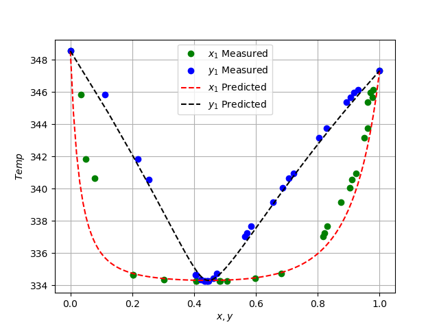
plt.figure(2)
plt.plot(x1_data, temp_data, "go")
plt.plot(y1_data, temp_data, "bo")
plt.plot(x1_linspace, T_predicted, "r--",)
plt.plot(y1_predicted, T_predicted, "k--",)
plt.legend(["$x_1$ Measured", "$y_1$ Measured", \
"$x_1$ Predicted", "$y_1$ Predicted"])
plt.xlabel("$x, y$")
plt.ylabel("$Temp$")
plt.grid()
plt.show()
Background on Parameter Estimation
A common application of optimization is to estimate parameters from experimental data. One of the most common forms of parameter estimation is the least squares objective with (model-measurement)^2 summed over all of the data points. The optimization problem is subject to the model equations that relate the model parameters or exogenous inputs to the predicted measurements. The model predictions are connected by common parameters that are adjusted to minimize the sum of squared errors.
Tutorial on Parameter Estimation
Nonlinear Confidence Interval
Nonlinear confidence intervals can be visualized as a function of 2 parameters. In this case, both parameters are simultaneously varied to find the confidence region. The confidence interval is determined with an F-test that specifies an upper limit to the deviation from the optimal solution
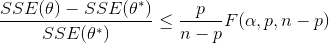
with p=2 (number of parameters), n=number of measurements, theta=[parameter 1, parameter 2] (parameters), theta* as the optimal parameters, SSE as the sum of squared errors, and the F statistic that has 3 arguments (alpha=confidence level, degrees of freedom 1, and degrees of freedom 2). For many problems, this creates a multi-dimensional nonlinear confidence region. In the case of 2 parameters, the nonlinear confidence region is a 2-dimensional space. Below is an example that shows the confidence region for the dye fading experiment confidence region for forward and reverse activation energies.
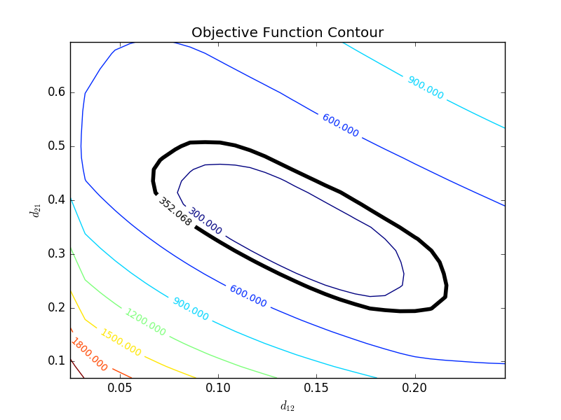
The optimal parameter values are in the 95% confidence region. This plot demonstrates that the 2D confidence region is not necessarily symmetric.
