TCLab Convective Heat Transfer
 |  |  |  |  |
|---|
Objective: Simulate an energy balance model with convective heat transfer.
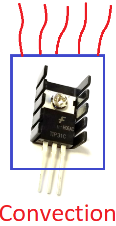
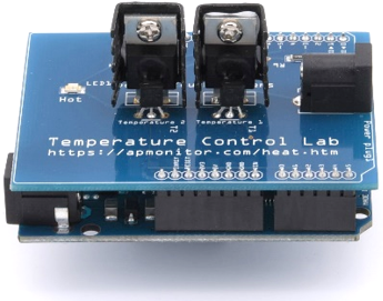
A basic energy balance model of the Temperature Control Lab (TCLab) assumes that there is one uniform temperature in the control volume and that all heat loss is through natural convection with U=10 W/m2-K. The relationship between the heater and the power output is given by `\alpha`=0.01 W/%.
$$m \, c_p \, \frac{dT}{dt} = U\,A\, \left(T_a-T\right) + \alpha \, Q$$
With the temperature initially at ambient temperature (`T_a`), simulate the change in temperature over the 5 minutes when heater Q is adjusted to 50%. Use values of m=0.004 kg, A=0.0012 m2, `c_p`=500 J/kg-K, and `T_a`=23 oC. Compare the simulated temperature response to data from the TCLab. Add a simulation prediction to the script below to compare with the TCLab data.
TCLab Step Response
import matplotlib.pyplot as plt
import tclab
import time
n = 300 # Number of second time points (5 min)
tm = np.linspace(0,n,n+1) # Time values
# data
lab = tclab.TCLab()
T1 = [lab.T1]
lab.Q1(50)
for i in range(n):
time.sleep(1)
print(lab.T1)
T1.append(lab.T1)
lab.close()
# Plot results
plt.figure(1)
plt.plot(tm,T1,'r.',label='Measured')
plt.ylabel('Temperature (degC)')
plt.xlabel('Time (sec)')
plt.legend()
plt.show()
Solutions
import matplotlib.pyplot as plt
from scipy.integrate import odeint
import tclab
import time
n = 300 # Number of second time points (5 min)
tm = np.linspace(0,n,n+1) # Time values
# data
lab = tclab.TCLab()
T1 = [lab.T1]
lab.Q1(50)
for i in range(n):
time.sleep(1.0)
print(lab.T1)
T1.append(lab.T1)
lab.close()
# simulation
def labsim(TC,t):
U = 10.0
A = 0.0012
Cp = 500
m = 0.004
alpha = 0.01
Ta = 23
dTCdt = (U*A*(Ta-TC) + alpha*50)/(m*Cp)
return dTCdt
Tsim = odeint(labsim,23,tm)
# Plot results
plt.figure(1)
plt.plot(tm,Tsim,'b-',label='Simulated')
plt.plot(tm,T1,'r.',label='Measured')
plt.ylabel('Temperature (degC)')
plt.xlabel('Time (sec)')
plt.legend()
plt.show()
import matplotlib.pyplot as plt
import tclab
import time
# pip install gekko
from gekko import GEKKO
n = 300 # Number of second time points (5 min)
# data
lab = tclab.TCLab()
T1 = [lab.T1]
lab.Q1(50)
for i in range(n):
time.sleep(1)
print(lab.T1)
T1.append(lab.T1)
lab.close()
# simulation
m = GEKKO()
m.time = np.linspace(0,n,n+1)
U = 10.0; A = 0.0012; Cp = 500
mass = 0.004; alpha = 0.01; Ta = 23
TC = m.Var(23)
m.Equation(mass*Cp*TC.dt()==U*A*(Ta-TC)+alpha*50)
m.options.IMODE = 4 # dynamic simulation
m.solve(disp=False)
# Plot results
plt.figure(1)
plt.plot(m.time,TC,'b-',label='Simulated')
plt.plot(m.time,T1,'r.',label='Measured')
plt.ylabel('Temperature (degC)')
plt.xlabel('Time (sec)')
plt.legend()
plt.show()
Generative AI Learning
Use these prompts to test your understanding after completing the exercise. Direct the AI - do not let it do the exercise for you.
App: Fit the convective energy balance in the browser with the TCLab Simulation Studio - choose the convective model, record a step test, and move the U and alpha sliders until the prediction matches the measurement; watch the sum-of-absolute-errors objective as you tune.
What to Turn In
Submit a short report (PDF, 1-2 pages) that curates your results into a demonstration of what you learned. You may use Generative AI to help write the report, but you must guide it to the correct visualizations, justifications, and assumptions. Answer these questions:
- Include the plot of predicted vs measured temperature. What U value (and alpha, if adjusted) gave the best fit in the app or your simulation, and how does it compare to the U=10 W/m2-K starting estimate?
- Compute the steady-state temperature predicted by the energy balance at Q=50% and show whether your data supports it.
- Which assumption of the lumped model (uniform temperature, constant U, no radiation) is most questionable at higher temperatures, and what evidence do you have?
- From the quiz prompt: one question you missed and the corrected answer.