Dynamics and Control

Optimization deals with selecting the best option among a number of possible choices that are feasible or don't violate constraints. Python can be used to optimize parameters in a model to best fit data, increase profitability of a potential engineering design, or meet some other type of objective that can be described mathematically with variables and equations.

Mathematical optimization problems may include equality constraints (e.g. =), inequality constraints (e.g. <, <=, >, >=), objective functions, algebraic equations, differential equations, continuous variables, discrete or integer variables, etc. A general statement of an optimization problem with nonlinear objectives or constraints is given by the following:

$$\mathrm{minimize} \quad J(x)$$ $$\mathrm{subject\;to}\quad g(x)>0$$ $$\quad\quad\quad\quad f(x)=0$$

The Karush Kuhn Tucker conditions must be satisfied in order to verify that a potential solution is optimal. An optimization problem has an objective J(x), n inequality constraints g(x), and m equality constraints f(x):

$$\min_x J(x)$$ $$\mathrm{subject\;to}\quad g_i(x) \ge 0 \quad i=1,\ldots,n$$ $$\quad\quad\quad\quad\quad f_i(x) = 0 \quad i=1,\ldots,m$$

There are four KKT conditions for optimal primal `(x)` and dual `(\lambda)` variables. A dual variable is a shadow price that shows how much the objective function can be locally improved if that constraint did not exist. The asterisk (*) is an indication that it is an optimal value.

1. Feasible Constraints

$$g_i(x^*) \mathrm{\;and\;} f_i(x^*) \mathrm{\;are\;feasible}$$

2. No Feasible Descent

$$\nabla J(x^*)-\sum_{i=1}^n \lambda_i^* \nabla g_i\left(x^*\right)-\sum_{i=1}^m \lambda_i^* \nabla f_i\left(x^*\right)=0$$

3. Complementary Slackness

$$\lambda_i^* \left( g_i(x^*) \right) = 0$$

4. Positive Lagrange Multipliers

$$\lambda_i^* \ge 0$$

Fortunately, there are good numerical methods for solving nonlinear programming problems to satisfy the KKT conditions. Three shown below are the APMonitor Optimization Suite (web interface), Python minimize function, and Python Gekko.

Exercise

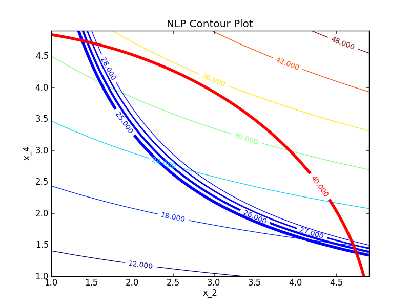
One example of an optimization problem from a benchmark test set is the Hock Schittkowski problem #71.

$$\min x_1 x_4 \left(x_1 + x_2 + x_3\right) + x_3$$ $$\mathrm{s.t.} \quad x_1 x_2 x_3 x_4 \ge 25$$ $$x_1^2 + x_2^2 + x_3^2 + x_4^2 = 40$$ $$1\le x_1, x_2, x_3, x_4 \le 5$$ $$x_0 = (1,5,5,1)$$

This problem has a nonlinear objective that the optimizer attempts to minimize. The variable values at the optimal solution are subject to (s.t.) both equality (=40) and inequality (>25) constraints. The product of the four variables must be greater than 25 while the sum of squares of the variables must also equal 40. In addition, all variables must be between 1 and 5 and the initial guess is x₁ = 1, x₂ = 5, x₃ = 5, and x₄ = 1.

For this problem determine:

1. A potential feasible solution
2. Identify the constraints on the contour plot
3. Mark the set of feasible solutions on the contour plot
4. Identify the minimum objective feasible solution
5. Identify the maximum objective feasible solution
6. Use a nonlinear programming solver to find a solution

Optimize with SciPy Minimize

Optimize with Gekko